
Code_Aster
®
Version
7.3
Titrate:
Law of behavior CAM-CLAY
Date:
03/02/05
Author (S):
J. EL GHARIB, G. DEBRUYNE
Key:
R7.01.14-B
Page
:
1/34
Manual of Reference
R7.01 booklet: Modelings for the Civil Engineering and the géomatériaux ones
HT-66/05/002/A
Organization (S):
EDF-R & D/AMA
Manual of Reference
R7.01 booklet: Modelings for the Civil Engineering and the géomatériaux ones
Document: R7.01.14
Law of behavior CAM-CLAY
Summary:
The Camwood-Clay model one of the elastoplastic models known and the most are the most used in mechanics of
grounds. It is especially adapted to argillaceous materials. There are several types of models Camwood-Clay, that
presented here is most current and is called modified Camwood-Clay. This model is characterized by surfaces of
load hammer-hardenable in the shape of ellipses in the diagram of the first two invariants of the stresses. With
the interior of these surfaces of reversibility, the material is elastic nonlinear. There exists moreover, in a point of
each ellipse, a critical state characterized by a null variation of volume. The whole of these points
constitute a line separating the areas from dilatancy and contractance from material as well as the areas
of negative and positive work hardening. Work hardening is governed by only one scalar variable and the rule of flow
normal is adopted.
Code_Aster
®
Version
7.3
Titrate:
Law of behavior CAM-CLAY
Date:
03/02/05
Author (S):
J. EL GHARIB, G. DEBRUYNE
Key:
R7.01.14-B
Page
:
2/34
Manual of Reference
R7.01 booklet: Modelings for the Civil Engineering and the géomatériaux ones
HT-66/05/002/A
1 Notations
indicate the tensor of the effective stresses in small disturbances defined as being
difference between the total stresses and the pressure of water in the case of water-logged soils, noted under
the shape of the following vector:
31
23
12
33
22
11
2
2
2
One notes:
()
tr
P
3
1
-
=
stress of containment
Pi
S
+
=
diverter of the stresses
()
S
S
tr
I
.
2
1
2
=
second invariant of the stresses
2
3I
Q
eq
=
=
equivalent stress
(
)
U
U
T
+
=
2
1
total deflection
HT
p
E
+
+
=
partition of the deformations (elastic, plastic, thermal)
()
(
)
0
3
T
T
tr
v
-
+
-
=
voluminal total deflection
()
p
p
V
tr
-
=
voluminal plastic deformation
I
v
3
1
~
+
=
diverter of the deformations
p
E
~
~
~
-
=
diverter of the elastic strain
I
p
v
p
p
3
1
~
+
=
deviatoric plastic deformation
(
)
E
E
E
eq
tr
~
.
~
3
2
=
equivalent elastic strain
(
)
p
p
p
eq
tr
~
.
~
3
2
=
equivalent plastic deformation

Code_Aster
®
Version
7.3
Titrate:
Law of behavior CAM-CLAY
Date:
03/02/05
Author (S):
J. EL GHARIB, G. DEBRUYNE
Key:
R7.01.14-B
Page
:
3/34
Manual of Reference
R7.01 booklet: Modelings for the Civil Engineering and the géomatériaux ones
HT-66/05/002/A
E
index of the vacuums of the material (report/ratio of the volume of the pores on the volume of the solid matter constituents)
0
E
initial index of the vacuums
porosity (report/ratio of the volume of the pores on total volume)
coefficient of swelling (elastic slope in a hydrostatic test of compression)
M
critical line slope of state
)
1
(
0
0
E
K
+
=
Cr
P
variable interns model, critical pressure equal to half of the pressure of consolidation
IDIOT
P
coefficient of compressibility (plastic slope in a hydrostatic test of compression)
)
(
)
1
(
0
-
+
=
E
K
µ
elastic coefficient of shearing (coefficient of Lamé)
F
surface of load
plastic multiplier
D
I
tensor unit of command 2 whose term running is
ij
D
I
4
tensor unit of command 4 whose term running is
ijkl

Code_Aster
®
Version
7.3
Titrate:
Law of behavior CAM-CLAY
Date:
03/02/05
Author (S):
J. EL GHARIB, G. DEBRUYNE
Key:
R7.01.14-B
Page
:
4/34
Manual of Reference
R7.01 booklet: Modelings for the Civil Engineering and the géomatériaux ones
HT-66/05/002/A
2 Introduction
The model describes here is the model known as of modified Camwood-Clay. The initial Camwood-Clay model was
developed by the school of soil mechanics of Cambridge in the Sixties. It predicted
too important deviatoric deformations under weak loading deviatoric, and was modified by
Burland and Roscoe in 1968 [bib1].
2.1
Phenomenology of the behavior of the grounds
The materials poroplastic such as certain clays are characterized by the behaviors
following:
·
the strong porosity of these materials causes unrecoverable deformations under loading
hydrostatic corresponding to an important reduction of porosity. This mechanism
purely contractor is sometimes called “collapse”,
·
under loading deviatoric, these materials show a contracting phase followed of one
phase where the material becomes deformed with constant plastic volume or dilates.
For the two types of loading, the energy locked in material evolves/moves according to the number
of contact between the grains. For a hydrostatic loading, the number of contact increases, thus
that locked energy, one thus has positive work hardening. For a loading deviatoric, the material
can become deformed without variation of volume to a number of intergranular contacts constant. Moreover,
one can observe in the tests of the localizations of deformations accompanied by strong
dilatancy. In these areas, the number of grains in decreasing contact, there is reduction in energy
locked and thus softening.
These behaviors are highlighted primarily by triaxial compression tests of revolution. These
observations bring to postulate that there is a plastic threshold whose evolution is controlled by two
mechanisms: one purely contractor associated with the hydrostatic stress, and a mechanism
deviatoric controlled by internal friction being held with constant volume and possibly
dilating with the approach of the localization.
All the interest of the Camwood Clay model lies in its faculty to describe these phenomena with one
minimum of products and in particular only one surface of load and a work hardening associated with one
only scalar variable.
2.2
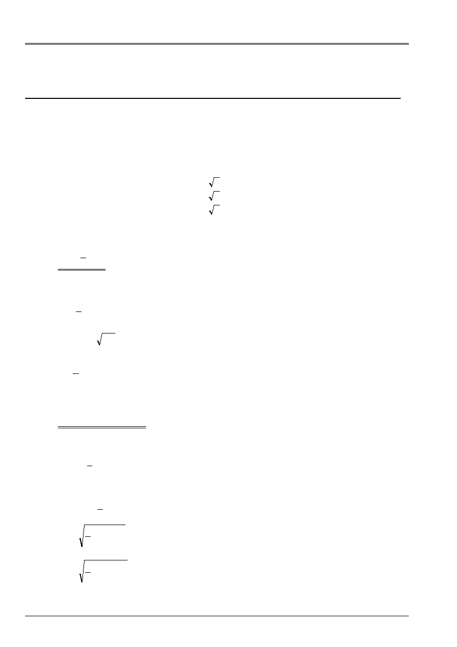
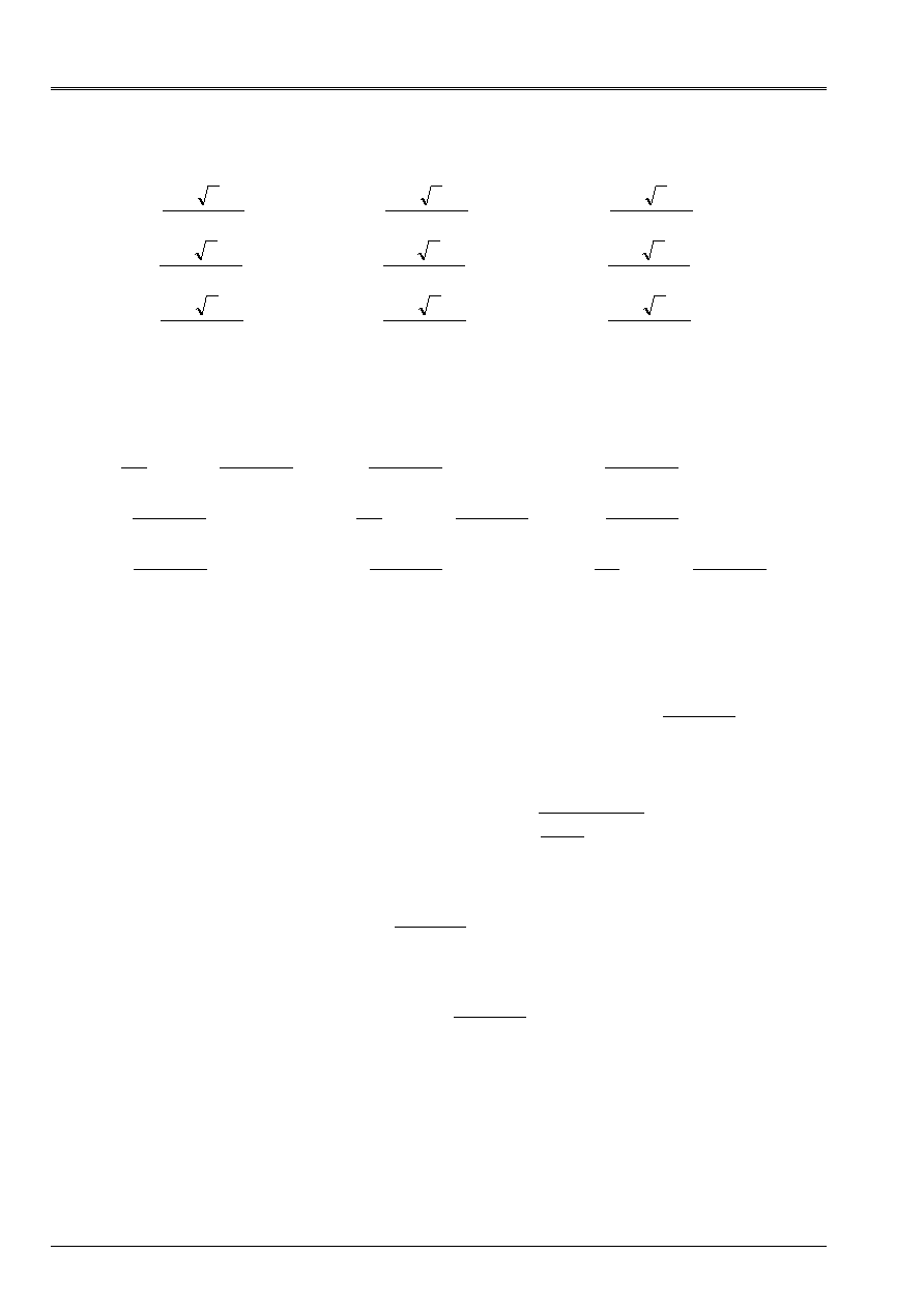
Behavior under hydrostatic compression
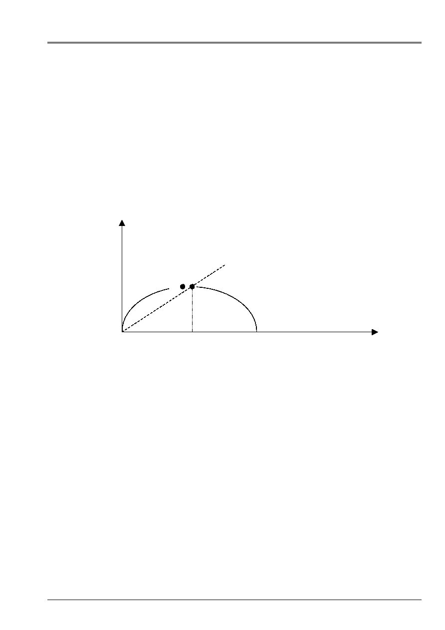
During a hydrostatic test of compression (
0
E
the initial index of the vacuums under loading equal to
atmospheric pressure
has
P
), the grounds present an index of the vacuums which decrease logarithmiquement
with the exerted hydrostatic pressure (cf [Figure 2.2-a]). Until a pressure
0
IDIOT
P
called
pressure of consolidation, the behavior is reversible, the slope
diagram
)
,
(
P
Ln
E
is
called elastic coefficient of swelling.
0
IDIOT
P
corresponds to the maximum pressure which underwent it
material during its history. Beyond this preconsolidation, the diagram presents one
new slope
(coefficient of compressibility) more marked and appearance of deformations
irreversible.
0
IDIOT
P
thus corresponds to an evolutionary elastoplastic threshold.
Code_Aster
®
Version
7.3
Titrate:
Law of behavior CAM-CLAY
Date:
03/02/05
Author (S):
J. EL GHARIB, G. DEBRUYNE
Key:
R7.01.14-B
Page
:
5/34
Manual of Reference
R7.01 booklet: Modelings for the Civil Engineering and the géomatériaux ones
HT-66/05/002/A
Appear 2.2-a: hydrostatic Test of loading and unloading
Note:
The diagram above corresponds to a whole of measurements where the effective stress is
stabilized. Indeed, in the process of consolidation of the grounds, it is the water contained in
the pores which takes again initially the hydrostatic pressure with very little deformation, front
to run out and let the skeleton become deformed. After consolidation of material and
stabilization of the pressure of water, the effective stress (forced total minus pressure
water) is stabilized and deferred on the graph. Relations of behavior in
saturated porous environments are generally expressed with the effective stresses according to
the assumption of Terzaghi.
2.3
Behavior under loading deviatoric
The triaxial compression tests of revolution make it possible to control at the same time the deviatoric component
Q
and
spherical component
P
loading. According to the report/ratio of these two components, one observes
a plastic behavior purely dilating (
M
P
Q
>
) or contracting (
M
P
Q
<
), line
Cr
MP
Q
=
representing the whole of the critical points on surfaces of load where the mechanical state evolves/moves
without plastic change of volume. The basic Camwood Clay model makes the assumption that the rates
plastic deformations are normal on the surface of load
F
(
Q
F
P
F
p
p
v
=
=
&
&
&
&
~
,
). Of
more, plastic work in an unspecified point of the surface of load is considered equal to work
plastic in a critical state. These considerations bring to the following equation for the plastic threshold:
0
)
(
)
,
,
(
=
+
=
Cr
Cr
P
P
Ln
MP
Q
P
Q
P
F
éq
2.3-1
Note:
In Code_Aster, the adopted criterion is that of modified the Cam_Clay model [éq 3.2-1].
Ln P
E
Ln
0
IDIOT
P
Ln AP
E
0
1
IDIOT
P
Ln
Code_Aster
®
Version
7.3
Titrate:
Law of behavior CAM-CLAY
Date:
03/02/05
Author (S):
J. EL GHARIB, G. DEBRUYNE
Key:
R7.01.14-B
Page
:
6/34
Manual of Reference
R7.01 booklet: Modelings for the Civil Engineering and the géomatériaux ones
HT-66/05/002/A
3
Camwood Clay law modified
The criterion of plasticity formulated above is not satisfactory for certain paths of loading.
In particular, for low values of
P
Q/
, the model predicts deviatoric deformations too much
important. To cure it, a new expression of plastic work was adopted, which
conduit with the model known as of Camwood modified Clay [bib1].
3.1
Assumptions of modeling
The model is written in small disturbances.
The coefficients of the model do not depend on the temperature.
3.2
Surface of load
The new assumptions lead to the following expression of the surface of load:
Cr
Cr
PP
M
P
M
Q
P
Q
P
F
2
2
2
2
2
)
,
,
(
-
+
=
0
éq
3.2-1
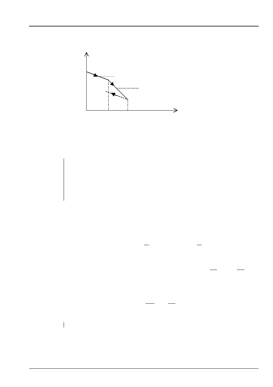
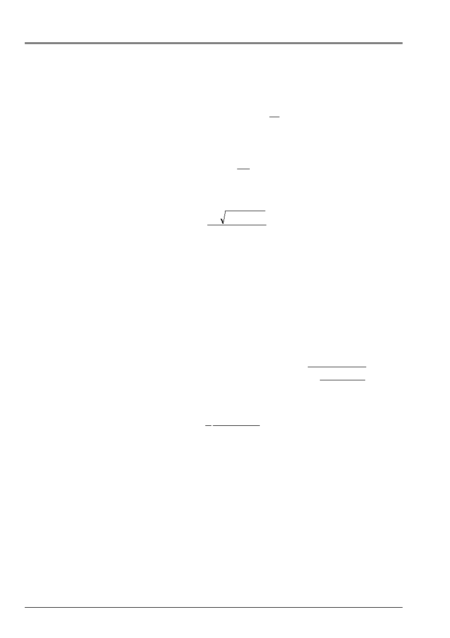
In the plan
)
,
(
Q
P
, the expression represents a family of ellipses, centered on
Cr
P
who is equal to
half of the pressure of consolidation (cf [Figure 3.2-a).
Cr
P
will be the parameter of work hardening of
model.
When
0
=
F
and
Cr
P
P
<
the material is dilating (
0
<
p
v
&
) and
Cr
P
is decreasing (softening).
When
0
=
F
and
Cr
P
P
>
the material is contacting (
0
>
p
v
&
) and
Cr
P
is increasing (hardening).
P
Q
Q=MP
Pcr1 Pcr2
Pcon1
Pcon2
Appear 3.2-a: Family of hammer-hardenable surfaces of load
Code_Aster
®
Version
7.3
Titrate:
Law of behavior CAM-CLAY
Date:
03/02/05
Author (S):
J. EL GHARIB, G. DEBRUYNE
Key:
R7.01.14-B
Page
:
7/34
Manual of Reference
R7.01 booklet: Modelings for the Civil Engineering and the géomatériaux ones
HT-66/05/002/A
3.3
Elastic law and law of work hardening
One makes the assumption of the decoupling of the partly hydrostatic and deviatoric elastic law and
the additional assumption that the modulus of rigidity is constant.
One thus considers an isotropic elastic law, with a linear deviatoric part and a part
voluminal non-linear:
Déviatoire part
:
µ
2
~
S
E
=
éq 3.3-1
Voluminal part
:
tion
Pconsolida
P
if
or
<
-
=
+
-
=
P
E
E
E
E
E
v
ln
1
0
0
&
&
éq 3.3-2
The law [éq 3.3-2] is in fact derived from a test oedometric where one measures the variation of the index of
vacuums according to the loading [Figure 2.2-a]. Let us recall that a homogeneous test oedometric
consist in increasing the axial effective stress all while maintaining the stress radial null on
a cylindrical test-tube.
Note:
Pressures
P
correspond to tests drained or not. Nevertheless, in one
modeling with Code_Aster stresses handled in the laws of behavior
are effective i.e. that one does not take into account the hydrostatic pressure of the fluid
who can circulate in the pores, the aforementioned being calculated in modelings THM.
The tests of voluminal loading (cf [Figure 2.2-a]) bring us to the following elastic law:
[
]
(
)
0
0
0
0
1
)
(
exp
E
K
K
P
P
p
v
v
+
=
-
=
with
éq
3.3-3
In the same way, growth of the surface of load in phase of contractance (and decrease for
the experimental dilatancy) and results suggest writing:
[
]
(
)
)
(
1
,
)
(
exp
0
0
0
-
+
=
-
=
E
K
K
P
P
p
v
p
v
Cr
Cr
with
éq
3.3-4
p
v
0
and
0
E
correspond to the voluminal deformation and the index of the initial vacuums, determined by
extrapolation of the oedometric curve of the test to the pressure
0
P
(cf [Figure 2.2-a]).
Code_Aster
®
Version
7.3
Titrate:
Law of behavior CAM-CLAY
Date:
03/02/05
Author (S):
J. EL GHARIB, G. DEBRUYNE
Key:
R7.01.14-B
Page
:
8/34
Manual of Reference
R7.01 booklet: Modelings for the Civil Engineering and the géomatériaux ones
HT-66/05/002/A
3.4
Plastic law of flow
The two plastic variables are the voluminal plastic deformation
p
v
and the tensor deviatoric
plastic deformations
p
~
. The internal variable is also
p
v
but associated the force
of work hardening
Cr
P
. The material standard is not generalized. The rule of flow is written:
Cr
p
v
p
P
F
F
-
=
=
&
&
&
&
,
,
,
éq
3.4-1
by breaking up the first term, one obtains:
Cr
p
v
p
p
v
P
F
S
F
P
F
-
=
=
=
&
&
&
&
&
&
~
éq 3.4-2
knowing that:
()
()
(
)
0
3
3
1
and
T
T
tr
tr
P
v
-
+
-
=
-
=
éq
3.4-3
F
is the plastic potential associated the phenomenon of work hardening. Let us note that the third part of
[éq 3.4-2] is only formal. Indeed, one knows
p
v
&
by the first relation thus one knows
evolution of
Cr
P
.
3.5
Energy writing and plastic module of work hardening
One is thus within the not generalized “standard” material framework (one uses three then
potentials: the surface of load
F
, plastic potential
F
, and free energy
. Even in this
configuration less favorable than the traditional framework of not generalized standard materials, one
is ensured to satisfy the second principle of thermodynamics [bib4]. Using the condition of
consistency (expressing that the point representative of the loading “follows” the surface of load) which
is written in the following way:
,
0
=
+
+
=
Cr
Cr
dP
P
F
dQ
Q
F
dP
P
F
df
éq
3.5-1
the expression of the plastic multiplier is determined [bib4]:
Cr
Cr
p
p
dP
P
F
H
D
F
H
-
=
=
1
1
éq
3.5-2
with [bib4]:
E
écrouissag
of
modulate
is
where
p
Cr
p
v
Cr
p
H
P
F
P
F
H
,
2
2
=
éq
3.5-3
Code_Aster
®
Version
7.3
Titrate:
Law of behavior CAM-CLAY
Date:
03/02/05
Author (S):
J. EL GHARIB, G. DEBRUYNE
Key:
R7.01.14-B
Page
:
9/34
Manual of Reference
R7.01 booklet: Modelings for the Civil Engineering and the géomatériaux ones
HT-66/05/002/A
The identification of the first and third part of [éq 3.4-2] makes it possible to calculate
F
who is written:
(
)
P
P
P
M
dP
P
F
F
Cr
Cr
Cr
2
2
-
=
-
=
éq
3.5-4
Concept of work hardening being associated that of locked energy:
p
v
p
v
Cr
p
v
Cr
D
dP
P
2
2
=
=
thus
éq
3.5-5
where
is the density of free energy:
))
(
exp (
)
exp (
)
(
2
3
0
0
0
0
0
2
p
v
p
v
Cr
E
v
E
eq
K
K
P
K
K
P
µ
-
+
+
=
éq
3.5-6
By using them [éq 3.4-2], [éq 3.5-4] and [éq 3.5-6], one can fire according to [éq 3.5-3] the expression from
modulate plastic work hardening:
(
)
Cr
Cr
Cr
p
v
Cr
p
P
P
PP
km
P
F
P
F
H
-
=
=
4
2
2
4
éq
3.5-7
The module of work hardening is positive in phase of contractance
(
)
Cr
P
P
>
and negative in phase of
dilatancy
(
)
Cr
P
P
<
. For
Cr
P
P
=
, the behavior is plastic perfect and proceeds with volume
constant plastic.
3.6 Relations
incremental
The equation [éq 3.4-3] and the condition of consistency give the relations of flow:
+
-
=
dQ
PP
M
Q
dP
P
P
K
D
Cr
Cr
p
v
2
1
1
1
éq
3.6-1
(
)
-
+
=
dQ
P
P
PP
M
Q
dP
PP
M
Q
K
D
Cr
Cr
Cr
p
eq
4
2
2
1
éq
3.6-2
Q
S
D
D
p
eq
p
2
3
~
=
éq 3.6-3
The rearrangement of [éq 3.6-1] and [éq 3.6-2] led to:
(
)
Cr
p
v
p
eq
P
P
M
Q
D
D
-
=
2
éq 3.6-4
i.e. with the equation [éq 3.6-3],
(
)
Cr
p
v
p
P
P
M
S
D
D
-
=
2
2
3
~
éq 3.6-5

Code_Aster
®
Version
7.3
Titrate:
Law of behavior CAM-CLAY
Date:
03/02/05
Author (S):
J. EL GHARIB, G. DEBRUYNE
Key:
R7.01.14-B
Page
:
10/34
Manual of Reference
R7.01 booklet: Modelings for the Civil Engineering and the géomatériaux ones
HT-66/05/002/A
Particular case of the critical point:
For
Cr
P
P
F
=
=
and
0
:
0
=
Cr
P
&
,
0
=
p
V
&
. One deduces some, by considering the elastic law:
V
P
K
P
&
&
0
=
.
The condition of consistency gives us
0
=
Q&
.
3.7
Summary of the relations of behavior and the data of the model
3.7.1 Data and critical of the model
The data specific to the model are five:
The critical slope
M
,
the initial index of the vacuums
0
E
associated an initial pressure equalizes in general with the pressure
atmospheric,
the elastic coefficient of swelling
(which leads to
0
K
),
the plastic coefficient of compressibility:
(which leads to
K
),
initial critical pressure
0
Cr
P
equalize with half of the pressure of preconsolidation,
which it is necessary to add the conventional coefficient of Lamé
µ
and the thermal expansion factor
. The coefficient of Lamé
µ
is in fact calculated starting from the two elastic coefficients
,
E
provided
in data.
The number of data is relatively low, which makes the model very simple. One of the limitations more
visible of the model is the assumption of the alignment of the critical points on a line of slope
M
.
This is besides the expression of the concept of internal friction. One can also interpret the size
M
by connecting it to the angle of repose natural of Coulomb by the relation:
M
M
+
=
6
3
sin
. However one knows
that for very cohesive materials, this angle varies when the mean stress decreases. One
besides note that for a chock of
M
on a triaxial compression test with a certain mean stress,
one simulates well with this model the triaxial ones realized with a mean stress pitch too different
but one cannot correctly consider the bearings plastic for a broad range of pressure of
containment (cf [bib2]). It is thus necessary to readjust
M
for several ranges of stress
average.

Code_Aster
®
Version
7.3
Titrate:
Law of behavior CAM-CLAY
Date:
03/02/05
Author (S):
J. EL GHARIB, G. DEBRUYNE
Key:
R7.01.14-B
Page
:
11/34
Manual of Reference
R7.01 booklet: Modelings for the Civil Engineering and the géomatériaux ones
HT-66/05/002/A
3.7.2 Summary of the relations of behavior of the model
Elasticity
E
S
µ
~
2
=
éq 3.7.2-1
()
E
v
K
P
P
0
0
exp
=
éq
3.7.2-2
Plasticity
The criterion:
(
)
0
2
,
2
2
2
2
=
-
+
=
Cr
Cr
PP
M
P
M
Q
P
F
with
(
)
eq
Q
=
4
4
4
4
3
4
4
4
4
2
1
+
-
=
Q
S
Q
F
I
P
F
F
D
2
3
3
1
éq
3.7.2-3
thus:
S
p
=
&
&
3
~
éq 3.7.2-4
(
)
Cr
p
v
P
P
M
-
=
2
2
&
&
éq
3.7.2-5
Work hardening
()
(
)
(
)
0
0
exp
p
v
p
v
Cr
p
v
Cr
K
P
P
-
=
éq
3.7.2-6
Elastic behavior: If
0
<
F
or (
0
=
F
and
0
f&
) then:
0
=
Cr
P
&
éq 3.7.2-7
0
,
0
~
=
=
p
v
p
eq
&
&
éq
3.7.2-8
µ
&
&
~
2
=
S
éq 3.7.2-9
P
K
P
v
&
&
0
=
éq
3.7.2-10
Elastoplastic behavior: If
0
=
F
and
0
=
f&
then:
Cr
p
v
Cr
Cr
P
K
P
P
&
&
&
=
;
0
éq
3.7.2-11
Cr
p
P
P
S
=
if
&
&
3
~
éq
3.7.2-12
(
)
Cr
Cr
p
v
P
P
P
P
M
-
=
if
2
2
&
&
éq 3.7.2-13
Note:
·
From the only unknown factor
p
v
&
, one can deduce the other unknown factors
p
&~
and
Cr
P
&
.
·
If
Cr
P
P
=
:
0
=
p
v
&
,
v
Cr
P
K
P
P
Q
&
&
&
&
0
,
0
=
=
=
.

Code_Aster
®
Version
7.3
Titrate:
Law of behavior CAM-CLAY
Date:
03/02/05
Author (S):
J. EL GHARIB, G. DEBRUYNE
Key:
R7.01.14-B
Page
:
12/34
Manual of Reference
R7.01 booklet: Modelings for the Civil Engineering and the géomatériaux ones
HT-66/05/002/A
4
Numerical integration of the relations of behavior
4.1
Recall of the problem
For an increment of loading given and a whole of variables given (initial field of
displacement, stress and variable intern), one solves the discretized total system (2.2.2.2-1 of [bib3])
who seeks to satisfy the equilibrium equations.
The resolution of this system gives us
U
, therefore
. One thus seeks locally (in each
not Gauss) the increment of stress and variable interns agent with
and which satisfies
law of behavior.
The following notations are employed:
With
With
With
-
,
,
for the quantity evaluated at the known moment T, with
the moment
T
T
+
and its increment respectively. The equations are discretized in manner
implicit, i.e. expressed according to the unknown variables at the moment
T
T
+
.
4.2
Calculation of the stresses and variables internal
The elastic prediction of the deviatoric stress is written:
µ
~
2
+
=
-
S
S
E
éq
4.2-1
however one can always write
S
at the moment + as being:
E
S
S
µ
~
2
+
=
-
éq 4.2-2
These two equations enable us to deduce
S
according to
E
S
:
E
E
S
S
µ
µ
~
2
~
2
+
-
=
éq
4.2-3
p
E
S
S
µ
~
2
-
=
or
éq 4.2-4
While replacing
p
~
by its expression according to
p
v
, one obtains:
(
)
Cr
p
v
E
P
P
M
S
S
-
+
=
2
3
1
µ
éq 4.2-5
from where,
(
)
Cr
p
v
E
P
P
M
Q
Q
-
+
=
2
3
1
µ
éq
4.2-6

Code_Aster
®
Version
7.3
Titrate:
Law of behavior CAM-CLAY
Date:
03/02/05
Author (S):
J. EL GHARIB, G. DEBRUYNE
Key:
R7.01.14-B
Page
:
13/34
Manual of Reference
R7.01 booklet: Modelings for the Civil Engineering and the géomatériaux ones
HT-66/05/002/A
One writes
P
according to the hydrostatic elastic prediction:
There is the equation
:
(
)
(
)
p
v
v
K
P
P
-
=
0
0
exp
éq 4.2-7
By supposing that
0
K
is independent of the temperature, the incremental writing of this
equation is:
[
]
-
-
-
=
E
v
E
v
K
K
P
P
0
0
exp
éq 4.2-8
[
]
E
v
K
P
P
=
-
0
exp
éq 4.2-9
[
]
)
1
(exp
0
-
=
-
E
v
K
P
P
éq
4.2-10
In the same way one can write the expression of
E
P
according to
-
P
:
[
]
v
E
K
P
P
=
-
0
exp
éq 4.2-11
from where the expression of
P
at the moment + is:
[
]
p
v
E
K
P
P
-
=
0
exp
éq 4.2-12
In the incremental writing of
Cr
P
, the coefficient
K
does not depend on the temperature, one thus finds
the following expression:
(
)
[
]
0
0
exp
p
v
p
v
Cr
Cr
K
P
P
-
=
éq
4.2-13
[]
p
v
Cr
Cr
K
P
P
=
-
exp
éq 4.2-14
(
)
[
]
1
exp
-
=
-
p
v
Cr
Cr
K
P
P
éq
4.2-15
Summary:
(
)
0
,
,
-
Cr
E
E
P
P
S
F
in this case
0
=
Cr
P
that is to say
E
S
S
S
S
=
+
=
-
E
P
P
=
(
)
0
,
,
>
-
Cr
E
E
P
P
S
F
in this case
0
>
Cr
P
,
0
~
p
and
0
p
v
that is to say
p
E
S
S
µ
~
2
-
=
[
]
p
v
E
K
P
P
-
=
0
exp
[]
p
v
Cr
Cr
K
P
P
=
-
exp
Note:
The main unknown factor is
p
v
.
Code_Aster
®
Version
7.3
Titrate:
Law of behavior CAM-CLAY
Date:
03/02/05
Author (S):
J. EL GHARIB, G. DEBRUYNE
Key:
R7.01.14-B
Page
:
14/34
Manual of Reference
R7.01 booklet: Modelings for the Civil Engineering and the géomatériaux ones
HT-66/05/002/A
4.3
Calculation of the unknown factor
p
v
By deferring in the criterion the expressions of
P
and
Q
according to
E
P
and of
E
Q
and while using
the equation [éq 4.2-6]:
(
)
Cr
Cr
p
v
E
P
P
P
M
P
P
M
Q
2
)
(
3
1
2
2
2
2
-
-
+
-
=
µ
éq
4.3-1
[
]
[]
(
)
[
]
[
]
[]
(
)
p
v
Cr
p
v
E
p
v
E
p
v
Cr
p
v
E
p
v
E
K
P
K
P
K
P
K
P
K
P
M
M
Q
µ
-
-
-
-
-
+
-
=
-
-
exp
2
exp
exp
exp
exp
3
1
0
0
2
0
2
2
2
éq
4.3-2
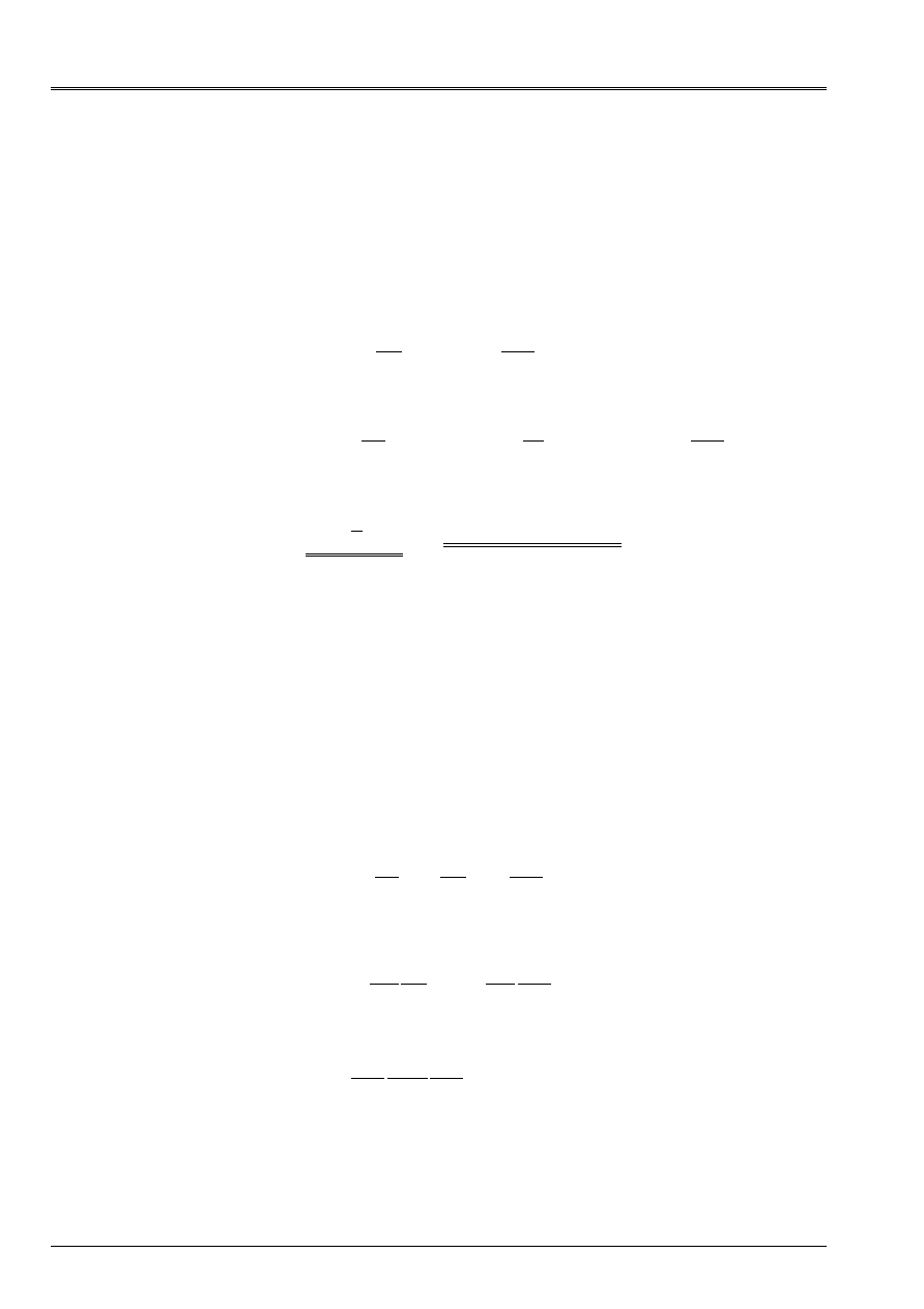
In under following paragraph one determines limits with this function which facilitate the resolution
equation [éq 4.3-2] with for example the method of the cords or by the method of Newton.
Some examples of paces of the preceding function are given in the following figures for
several data files.
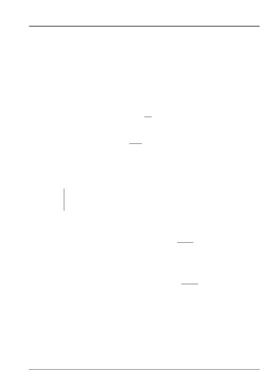
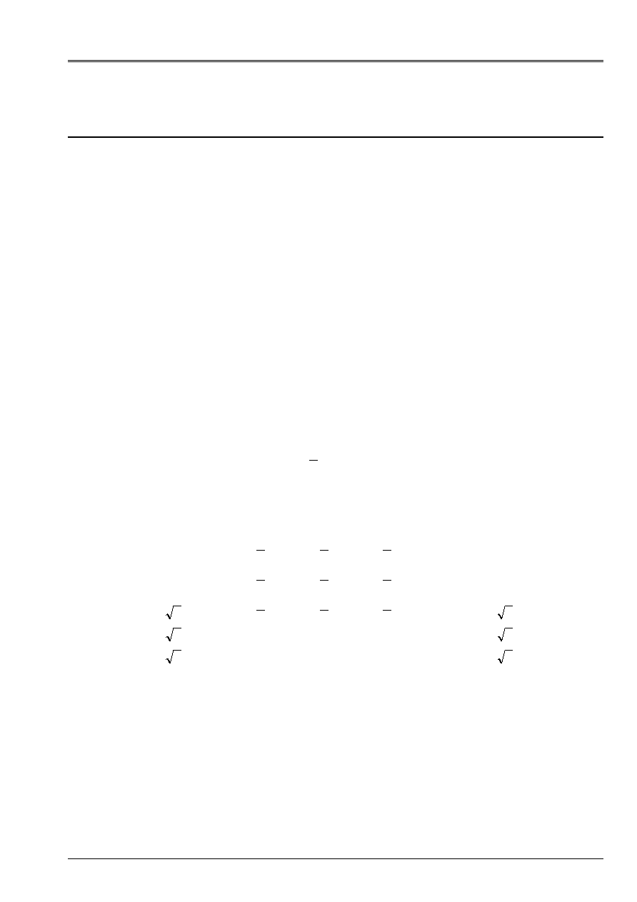
Particular case:
0
=
Q
(hydrostatic test of compression)
The criterion is reached for
Cr
P
P 2
=
From where:
(
)
(
)
p
v
Cr
p
v
E
K
P
K
P
=
-
-
exp
2
exp
0
Thus
-
+
=
Cr
E
p
v
P
P
Ln
K
K
2
1
0
For:
9
,
0
=
M
;
4000
=
µ
;
2
,
0
=
-
Cr
P
;
10
=
K
;
30
0
=
K
and
1
=
E
P
; then
3
310
.
2
-
=
p
v
Appear 4.3-a: Pace of the function [éq 4.3-2] for
0
=
Q
Code_Aster
®
Version
7.3
Titrate:
Law of behavior CAM-CLAY
Date:
03/02/05
Author (S):
J. EL GHARIB, G. DEBRUYNE
Key:
R7.01.14-B
Page
:
15/34
Manual of Reference
R7.01 booklet: Modelings for the Civil Engineering and the géomatériaux ones
HT-66/05/002/A
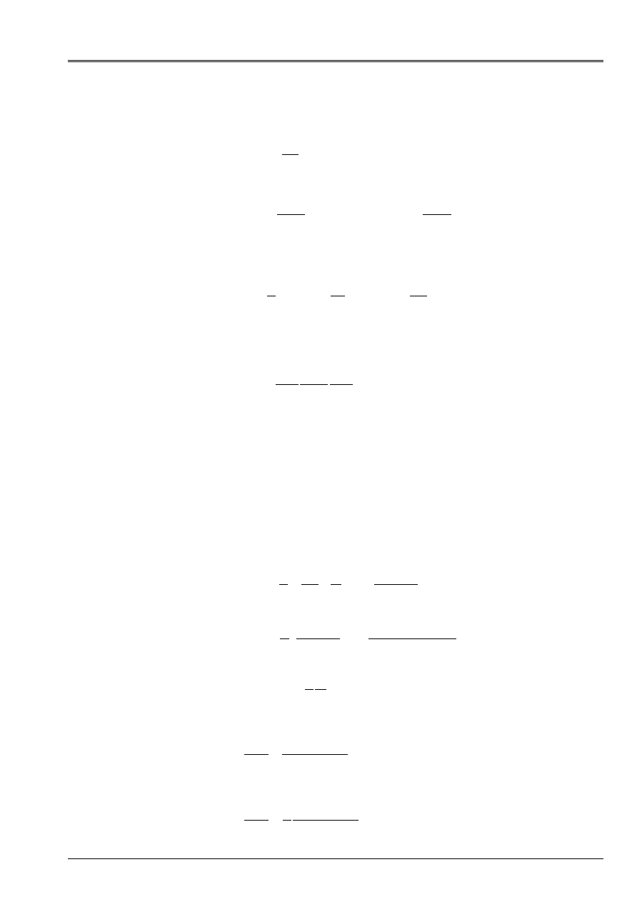
Example for:
-
-
<
MP
Q
(contractance)
That is to say following data:
9
,
0
=
M
;
4000
=
µ
;
2
,
0
=
-
Cr
P
;
10
=
K
;
30
0
=
K
2
=
E
Q
;
6
,
0
=
E
P
;
4
10
.
2
~
-
=
eq
;
4
10
.
3
-
=
v
Appear 4.3-b: Pace of the function [éq 4.3-2] for
-
-
<
MP
Q
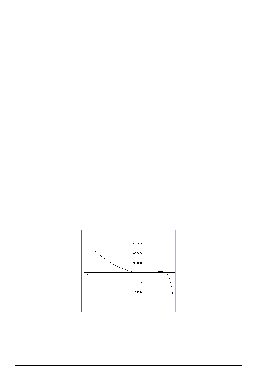
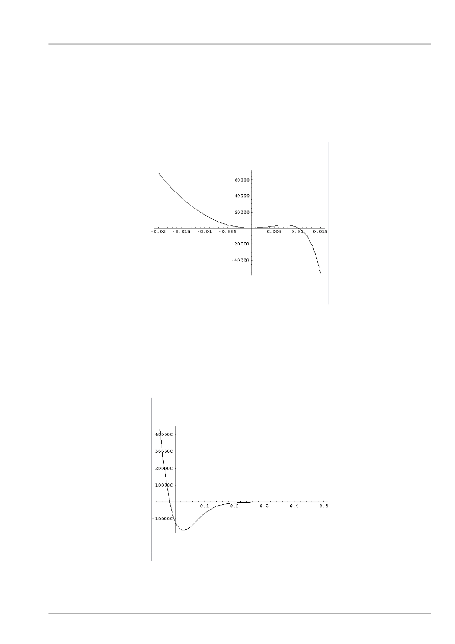
Example for:
-
-
>
MP
Q
(dilatancy)
That is to say following data:
9
,
0
=
M
;
4000
=
µ
;
2
,
0
=
-
Cr
P
;
10
=
K
;
30
0
=
K
2
=
E
Q
;
2
,
0
=
E
P
;
4
10
.
2
~
-
=
eq
;
4
10
.
3
-
=
v
Appear 4.3-c: Pace of the function [éq 4.3-2] for
-
-
>
MP
Q

Code_Aster
®
Version
7.3
Titrate:
Law of behavior CAM-CLAY
Date:
03/02/05
Author (S):
J. EL GHARIB, G. DEBRUYNE
Key:
R7.01.14-B
Page
:
16/34
Manual of Reference
R7.01 booklet: Modelings for the Civil Engineering and the géomatériaux ones
HT-66/05/002/A
4.4
Determination of the terminals of the function
One poses
X
p
v
=
the unknown factor of the problem.
One thus has:
(
)
X
K
P
X
P
E
0
exp
)
(
-
=
éq
4.4-1
)
exp (
)
(
kx
P
X
P
Cr
Cr
-
=
éq 4.4-2
()
(
)
X
P
X
P
M
X
X
Cr
-
=
)
(
2
)
(
2
éq
4.4-3
)
(
6
1
)
(
X
Q
X
Q
E
+
=
µ
éq 4.4-4
()
()
()
() ()
0
2
2
2
2
2
=
-
+
=
X
P
X
P
M
X
P
M
X
Q
X
F
Cr
éq
4.4-5
()
0
X
then two cases arise:
0
X
and
Cr
P
P
()
()
0
0
Cr
P
P
and
sup
0
X
X
;
()
()
sup
sup
X
P
X
P
Cr
=
éq
4.4-6
0
X
and
Cr
P
P
()
()
0
0
Cr
P
P
and
0
inf
X
X
;
()
()
inf
inf
X
P
X
P
Cr
=
éq
4.4-7
The first terminal is the 0 which is the terminal inf in the case of the contractance and limits it sup in
case of dilatancy.
Calculation of the second terminal
inf
sup
X
X
X
B
=
=
:
()
()
(
)
()
B
Cr
B
E
B
Cr
B
kx
P
X
K
P
X
P
X
P
exp
exp
0
-
=
-
=
(
)
-
-
+
=
+
=
Cr
E
B
B
Cr
E
P
P
Ln
K
K
X
X
K
K
P
P
0
0
1
exp
éq
4.4-8
One will thus distinguish between the two fields:
Dilatancy:
[]
0
;
B
X
X
and Contractance:
[
]
B
X
X
:
0
Values of the function at the boundaries:
Code_Aster
®
Version
7.3
Titrate:
Law of behavior CAM-CLAY
Date:
03/02/05
Author (S):
J. EL GHARIB, G. DEBRUYNE
Key:
R7.01.14-B
Page
:
17/34
Manual of Reference
R7.01 booklet: Modelings for the Civil Engineering and the géomatériaux ones
HT-66/05/002/A
At the point
()
()
E
Cr
Cr
E
Q
Q
P
P
P
P
X
=
=
=
=
=
-
0
;
0
0
;
)
0
(
;
)
0
(
;
0
éq
4.4-9
()
(
)
-
-
+
=
Cr
E
E
E
P
P
P
M
Q
F
2
0
2
2
éq
4.4-10
At the point
()
()
()
2
2
0
;
;
P
M
X
F
X
Q
X
P
P
X
X
B
B
B
Cr
B
-
=
=
=
=
=
and
éq 4.4-11
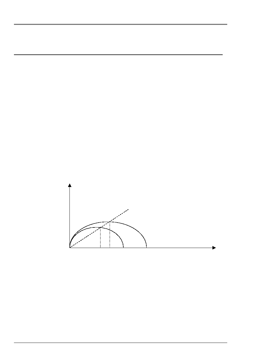
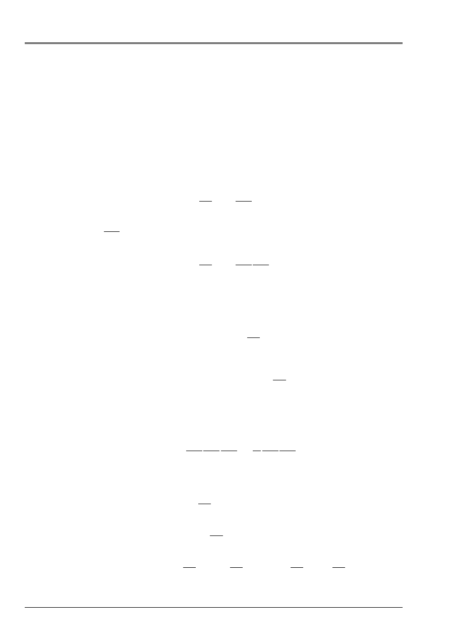
4.5
Particular case of the critical point
If at the moment
-
T
one reaches the critical state, then
0
,
=
=
-
+
p
v
Cr
Cr
P
P
and
-
-
=
MP
Q
. If
0
,
0
=
=
F
F
&
,
then the point
)
,
(Q
P
at the moment
+
T
moves on the initial ellipse (cf [Figure 4.5-a]). One deduces immediately from the law
rubber band and of the condition
0
=
p
v
:
-
=
P
K
P
v
0
éq 4.5-1
The criterion being checked at the moment
+
T
, one has while using [éq 4.5-1]:
)
1
(
)
1
(
)
) (
(
)
2
(
2
2
0
)
2
(
2
2
0
)
2
(
2
2
2
2
v
V
Cr
K
Q
K
P
M
P
P
P
P
M
P
P
P
M
Q
-
=
-
=
-
+
=
-
=
-
-
-
-
+
-
+
+
éq 4.5-2
T
+
T
-
P
Q
Q=MP
Pcr
Pcon
Appear mechanical 4.5-a: State around the critical point
Code_Aster
®
Version
7.3
Titrate:
Law of behavior CAM-CLAY
Date:
03/02/05
Author (S):
J. EL GHARIB, G. DEBRUYNE
Key:
R7.01.14-B
Page
:
18/34
Manual of Reference
R7.01 booklet: Modelings for the Civil Engineering and the géomatériaux ones
HT-66/05/002/A
In addition the diverter of the stresses can be written:
S
S
S
F
S
S
S
E
E
p
E
-
=
-
=
-
=
µ
µ
µ
6
2
~
2
éq
4.5-3
One deduces some:
Q
Q
E
=
+
µ
6
1
, éq
4.5-4
and:
E
E
V
S
Q
K
Q
S
2
2
0
1
(
-
=
-
éq
4.5-5
4.6 Summary
The discretization of the equations and the law of implicit behavior of manner leads to the resolution
equation [éq 4.3-2].
If
-
-
Cr
P
P
, then one solves the equation [éq 4.3-2] whose unknown factor is
p
v
.
One deduces then:
(
)
Cr
p
v
E
p
v
v
p
v
Cr
Cr
P
P
M
S
S
K
P
P
K
P
P
-
+
=
-
=
=
-
-
2
0
3
1
),
(
exp (
),
exp (
µ
then
éq 4.6-1
One deduces finally:
S
P
P
M
Cr
p
v
p
)
(
2
3
~
2
-
=
éq
4.6-2
At the critical point:
-
=
=
Cr
Cr
p
v
P
P
,
0
éq
4.6-3
In this point, there is no evolution of work hardening, on the other hand the state of stress can continue with
to evolve/move either in contractance, or in dilatancy (the tangent with the criterion is horizontal). The new state
stresses moves on the surface of load of the preceding state.
Code_Aster
®
Version
7.3
Titrate:
Law of behavior CAM-CLAY
Date:
03/02/05
Author (S):
J. EL GHARIB, G. DEBRUYNE
Key:
R7.01.14-B
Page
:
19/34
Manual of Reference
R7.01 booklet: Modelings for the Civil Engineering and the géomatériaux ones
HT-66/05/002/A
5 Operator
tangent
If the option is:
RIGI_MECA_TANG
, option used at the time of the prediction, the tangent operator calculated in
each point of Gauss is known as of speed:
kl
elp
ijkl
ij
D
&
&
=
In this case,
elp
ijkl
D
is calculated starting from the not discretized equations.
If the option is:
FULL_MECA
, option used when one reactualizes the tangent matrix with each iteration
by updating the internal stresses and variables:
kl
ijkl
ij
D
With
D
=
In this case,
ijkl
With
is calculated starting from the implicitly discretized equations.
5.1
Nonlinear elastic tangent operator
The elastic relation of speed is written:
µ
&
&
&
&
&
~
2
0
+
=
+
-
=
ij
ij
ij
ij
Ptr
K
S
P
éq
5.1-1
ij
ij
ij
tr
P
K
µ
µ
&
&
&
2
)
3
2
(
0
+
-
=
éq
5.1-2
The tangent operator in elasticity of the law noted Cam_Clay
E
D
is thus deduced from the matric writing
following:
+
-
-
-
+
-
-
-
+
=
31
23
12
33
22
11
0
0
0
0
0
0
0
0
0
31
23
12
33
22
11
2
2
2
2
0
0
0
0
0
0
2
0
0
0
0
0
0
2
0
0
0
0
0
0
3
4
3
2
3
2
0
0
0
3
2
3
4
3
2
0
0
0
3
2
3
2
3
4
2
2
2
µ
µ
µ
µ
µ
µ
µ
µ
µ
µ
µ
µ
&
&
&
&
&
&
4
4
4
4
4
4
4
4
4
4
3
4
4
4
4
4
4
4
4
4
4
2
1
&
&
&
&
&
&
E
D
P
K
P
K
P
K
P
K
P
K
P
K
P
K
P
K
P
K
éq 5.1-3
Code_Aster
®
Version
7.3
Titrate:
Law of behavior CAM-CLAY
Date:
03/02/05
Author (S):
J. EL GHARIB, G. DEBRUYNE
Key:
R7.01.14-B
Page
:
20/34
Manual of Reference
R7.01 booklet: Modelings for the Civil Engineering and the géomatériaux ones
HT-66/05/002/A
5.2
Plastic tangent operator of speed. Option
RIGI_MECA_TANG
The total tangent operator is in this case
1
-
I
K
(the option
RIGI_MECA_TANG
called with the first
iteration of a new increment of load) starting from the results known at the moment
1
-
I
T
[bib3].
If the tensor of the stresses with
1
-
I
T
is on the border of the field of elasticity, one writes the condition:
0
=
f&
who must be checked jointly with the condition
0
=
F
. If the tensor of the stresses with
1
-
I
T
is inside the field,
0
<
F
, then the tangent operator is the operator of elasticity.
0
=
+
=
Cr
Cr
P
P
F
F
F
&
&
&
éq
5.2-1
like
p
v
p
v
Cr
Cr
P
P
&
&
=
, then:
0
=
+
=
p
v
p
v
Cr
Cr
P
P
F
F
F
&
&
&
éq
5.2-2
In addition
p
E
&
&
&
-
=
thus:
-
=
-
F
D
E
&
&
&
1
,
éq
5.2-3
i.e.:
kl
E
ijkl
kl
E
ijkl
ij
F
D
D
-
=
&
&
&
éq
5.2-4
The plastic module of work hardening is written according to the equation [éq 3.5-7] and by using the rule
of flow:
p
v
p
v
Cr
Cr
Cr
p
v
Cr
Cr
p
P
P
F
P
F
P
P
F
H
&
&
-
=
=
1
éq
5.2-5
The equations [éq 5.2-1] and [éq 5.2-5] give:
0
=
-
p
ij
ij
H
F
&
&
éq
5.2-6
Multiplication of the equation [éq 5.2-4] by
ij
F
give:
kl
E
ijkl
ij
E
ijkl
ij
ij
ij
F
D
F
D
F
F
-
=
&
&
&
éq 5.2-7
Code_Aster
®
Version
7.3
Titrate:
Law of behavior CAM-CLAY
Date:
03/02/05
Author (S):
J. EL GHARIB, G. DEBRUYNE
Key:
R7.01.14-B
Page
:
21/34
Manual of Reference
R7.01 booklet: Modelings for the Civil Engineering and the géomatériaux ones
HT-66/05/002/A
The two preceding equations make it possible to find:
kl
E
ijkl
ij
kl
E
ijkl
ij
p
F
D
F
D
F
H
-
=
&
&
&
éq
5.2-8
from where the expression of the plastic multiplier:
p
kl
E
ijkl
ij
kl
E
ijkl
ij
H
F
D
F
D
F
+
=
&
&
éq
5.2-9
That is to say H the definite elastoplastic module like:
p
kl
E
ijkl
ij
H
F
D
F
H
+
=
éq
5.2-10
The plastic multiplier is written:
H
D
F
kl
E
ijkl
ij
&
&
=
éq
5.2-11
While replacing
&
by his expression in the equation [éq 5.2-4], one obtains:
kl
E
ijkl
COp
E
mnop
Mn
kl
E
ijkl
ij
F
D
D
F
H
D
-
=
.
1
&
&
&
éq
5.2-12
One thus deduces the elastoplastic operator from it
p
E
elp
D
D
D
-
=
:
kl
D
Mn
E
mnkl
E
ijop
COp
E
ijkl
ij
elp
F
D
D
F
H
D
&
4
4
4
4
4
4
4
3
4
4
4
4
4
4
4
2
1
&
-
=
1
éq 5.2-13
with,
Mn
E
mnkl
E
ijop
COp
p
ijkl
F
D
D
F
H
D
=
1
éq 5.2-14
Code_Aster
®
Version
7.3
Titrate:
Law of behavior CAM-CLAY
Date:
03/02/05
Author (S):
J. EL GHARIB, G. DEBRUYNE
Key:
R7.01.14-B
Page
:
22/34
Manual of Reference
R7.01 booklet: Modelings for the Civil Engineering and the géomatériaux ones
HT-66/05/002/A
Calculation of
H
:
(
)
ij
ij
Cr
ij
S
P
P
M
F
3
3
2
2
+
-
-
=
,
éq
5.2-15
who is written in vectorial notation:
(
)
(
)
(
)
+
-
-
+
-
-
+
-
-
31
23
12
33
2
22
2
11
2
2
3
2
3
2
3
3
3
2
3
3
2
3
3
2
S
S
S
S
P
P
M
S
P
P
M
S
P
P
M
Cr
Cr
Cr
éq
5.2-16
from where the expression of:
(
)
(
)
(
)
+
-
-
+
-
-
+
-
-
31
23
12
33
2
0
22
2
0
11
2
0
2
6
2
6
2
6
6
2
6
2
6
2
:
S
S
S
S
P
P
P
M
K
S
P
P
P
M
K
S
P
P
P
M
K
F
D
Cr
Cr
Cr
kl
E
ijkl
µ
µ
µ
µ
µ
µ
éq
5.2-17
and
2
2
4
0
12
)
(
4
Q
P
P
P
M
K
F
D
F
Cr
kl
E
ijkl
ij
µ
+
-
=
éq
5.2-18
According to the equations [éq 3.5-7] and [éq 5.2-17], one can deduce the expression from
H
:
(
) (
)
(
)
2
0
4
4
4
Q
kP
P
P
K
P
P
P
M
H
Cr
Cr
Cr
µ
+
+
-
-
=
éq 5.2-19
While posing:
(
)
ij
ij
Cr
ij
S
P
P
P
M
K
With
µ
6
2
2
0
+
-
-
=
,
éq
5.2-20
one can write the following symmetrical plastic matrix:
=
2
31
2
31
23
2
2
23
2
31
12
2
23
12
2
2
12
2
31
33
23
33
12
33
2
33
31
22
23
22
12
22
33
22
2
22
31
11
23
11
12
11
33
11
22
11
2
11
36
.
.
.
.
.
36
36
.
.
.
.
36
36
36
.
.
.
2
6
2
6
2
6
.
.
2
6
2
6
2
6
.
2
6
2
6
2
6
1
S
S
S
S
S
S
S
S
S
S
With
S
With
S
With
With
S
With
S
With
S
With
With
With
With
S
With
S
With
S
With
With
With
With
With
With
H
D
p
µ
µ
µ
µ
µ
µ
µ
µ
µ
µ
µ
µ
µ
µ
µ
éq
5.2-21

Code_Aster
®
Version
7.3
Titrate:
Law of behavior CAM-CLAY
Date:
03/02/05
Author (S):
J. EL GHARIB, G. DEBRUYNE
Key:
R7.01.14-B
Page
:
23/34
Manual of Reference
R7.01 booklet: Modelings for the Civil Engineering and the géomatériaux ones
HT-66/05/002/A
5.3
Tangent operator into implicit. Option
FULL_MECA
To calculate the tangent operator into implicit, one chose by preoccupation with a simplicity to separate in first
place processing of the deviatoric part of the hydrostatic part for then combining them in order to
to deduce the tangent operator connecting the disturbance from the total stress to the disturbance of
total deflection.
5.3.1 Processing of the deviatoric part
It is considered here that the variation of loading is purely deviatoric
)
0
(
=
P
.
The increment of the deviatoric stress is written in the form:
(
)
p
ij
ij
ij
S
µ
~
~
2
-
=
éq
5.3.1-1
Around the point of balance
(
)
+
-
, a variation is considered
S
deviatoric part of
stress:
(
)
p
kl
kl
kl
S
µ
~
~
2
-
=
éq
5.3.1-2
Calculation of
p
kl
~
:
It is known that:
kl
p
kl
S
=
3
~
éq
5.3.1-3
By deriving this equation compared to the deviatoric stress, one obtains:
kl
kl
p
kl
S
S
+
=
3
3
~
éq
5.3.1-4
Calculation of
:
One a:
(
)
[
]
P
P
P
M
S
S
H
P
P
F
S
S
F
H
F
H
Cr
Mn
Mn
p
Mn
Mn
p
Mn
Mn
p
-
+
=
+
=
=
2
2
3
1
1
1
éq 5.3.1-5
If one considers only the evolution of the deviatoric part of
)
0
(
=
P
, then:
[
]
Cr
Mn
Mn
Mn
Mn
p
p
p
P
P
M
S
S
S
S
H
H
H
-
+
=
+
=
2
2
3
3
)
(
éq
5.3.1-6
However:
P
v
Cr
Cr
kP
P
=
.
Cr
Cr
p
V
Cr
p
v
P
M
P
P
M
P
P
M
-
-
=
-
=
2
2
2
2
)
(
2
),
(
2
has
one
Like
, éq
5.3.1-7
From where:
.
2
1
)
(
2
2
2
Cr
Cr
Cr
P
M
kP
P
P
M
+
=
-
éq
5.3.1-8
Code_Aster
®
Version
7.3
Titrate:
Law of behavior CAM-CLAY
Date:
03/02/05
Author (S):
J. EL GHARIB, G. DEBRUYNE
Key:
R7.01.14-B
Page
:
24/34
Manual of Reference
R7.01 booklet: Modelings for the Civil Engineering and the géomatériaux ones
HT-66/05/002/A
In addition,
.
)
2
(
4
)
(
4
4
4
Cr
Cr
p
Cr
Cr
p
P
P
P
P
km
H
P
P
PP
km
H
-
=
-
=
and
éq 5.3.1-9
By injecting this last equation in the equation [éq 5.3.1-6], one obtains:
[
]
[
]
Mn
Mn
Mn
Mn
Cr
Cr
p
S
S
S
S
P
P
M
P
P
P
km
H
3
3
2
)
2
(
4
2
4
+
=
+
-
+
éq
5.3.1-10
While using the relation [éq 5.3.1-8], it comes then:
[
]
)
(
3
3
With
H
S
S
S
S
p
Mn
Mn
Mn
Mn
+
+
=
éq
5.3.1-11
with
[
]
+
-
+
-
=
2
2
2
4
2
1
)
(
2
)
2
(
4
M
kP
P
P
M
P
M
P
P
P
M
K
With
Cr
Cr
Cr
One then obtains immediately the variation of the deviatoric part of the plastic deformation:
(
)
(
)
kl
Cr
p
kl
Mn
Mn
p
kl
Mn
Mn
kl
Mn
Mn
p
p
kl
S
P
P
P
M
H
S
S
S
H
S
S
S
S
S
S
With
H
-
+
+
+
+
=
2
6
9
)
(
9
~
éq 5.3.1-12
ij
S
is written then:
(
)
[
]
(
)
ij
Cr
p
ij
kl
kl
p
kl
ij
kl
kl
ij
kl
p
ij
ij
S
P
P
P
M
H
S
S
S
H
S
S
S
S
S
S
With
H
S
µ
µ
µ
µ
-
-
-
+
+
-
=
2
12
18
)
(
18
~
2
éq 5.3.1-13
who becomes by separating the terms in variation from stresses and the term in variation of deformation
total:
(
)
(
)
ij
kl
ijkl
Mn
Mn
p
ij
kl
ij
kl
p
Cr
p
ijkl
ijkl
S
S
S
H
S
S
S
S
With
H
P
P
P
M
H
µ
µ
µ
µ
~
2
18
18
12
2
=
+
+
+
+
-
+
éq 5.3.1-14
or in tensorial writing:
(
)
µ
µ
µ
µ
~
2
)
(
)
(
18
:
18
12
1
2
4
=
+
+
+
+
-
+
S
S
S
S
With
H
S
S
H
P
P
P
M
H
I
p
p
Cr
p
D
éq 5.3.1-15
that one can still write by symmetrizing the tensor
S
S
S
+
)
(
:
(
)
µ
µ
µ
µ
~
2
)
(
18
:
18
12
1
2
4
=
+
+
+
-
+
S
With
H
S
S
H
P
P
P
M
H
I
p
p
Cr
p
D
éq 5.3.1-16
with:
[
]
T
S
S
S
S
S
S
))
(
(
)
)
((
2
1
+
+
+
=
Code_Aster
®
Version
7.3
Titrate:
Law of behavior CAM-CLAY
Date:
03/02/05
Author (S):
J. EL GHARIB, G. DEBRUYNE
Key:
R7.01.14-B
Page
:
25/34
Manual of Reference
R7.01 booklet: Modelings for the Civil Engineering and the géomatériaux ones
HT-66/05/002/A
Calculation of
, while posing:
ij
ij
ij
S
S
T
+
=
31
31
23
31
12
31
33
31
22
31
11
31
31
23
23
23
12
23
33
23
22
23
11
23
31
12
23
12
12
12
33
12
22
12
11
12
31
33
23
33
12
33
33
33
22
33
11
33
31
22
23
22
12
22
33
22
22
22
11
22
31
11
23
11
12
11
33
11
22
11
11
11
2
2
2
2
2
2
2
2
2
2
2
2
2
2
2
2
2
2
2
2
2
2
2
2
2
2
=
S
S
T
S
T
S
T
S
T
S
T
S
T
S
T
S
T
S
T
S
T
S
T
S
T
S
T
S
T
S
T
S
T
S
T
S
T
S
T
S
T
S
T
S
T
S
T
S
T
S
T
S
T
S
T
S
T
S
T
S
T
S
T
S
T
S
T
S
T
S
T
S
T
T
éq 5.3.1-17
[
]
T
S
T
S
T
)
(
)
(
2
1
+
=
éq 5.3.1-18
That is to say:
(
)
+
+
+
-
+
=
)
(
9
:
9
6
2
1
2
4
With
H
S
S
H
P
P
P
M
H
I
C
p
p
Cr
p
D
µ
éq 5.3.1-19
one poses:
(
)
S
S
H
C
p
:
9
=
éq 5.3.1-20
and
(
)
P
P
P
M
H
D
Cr
p
-
=
2
6
éq 5.3.1-21
The symmetrical matrix
C
dimensions (6,6) is too large to be presented whole, one
break up into 4 parts
1
C
,
2
C
,
3
C
and
4
C
:
=
4
3
2
1
C
C
C
C
C
with
+
+
+
+
+
+
+
+
+
+
+
+
+
+
+
+
+
+
+
+
+
+
+
+
=
33
33
22
33
33
22
33
11
11
33
22
33
33
22
22
22
22
11
11
22
11
33
33
11
11
22
22
11
11
11
1
)
(
9
2
1
)
(
)
(
2
9
)
(
)
(
2
9
)
(
)
(
2
9
)
(
9
2
1
)
(
)
(
2
9
)
(
)
(
2
9
)
(
)
(
2
9
)
(
9
2
1
S
T
With
H
D
C
S
T
S
T
With
H
S
T
S
T
With
H
S
T
S
T
With
H
S
T
With
H
D
C
S
T
S
T
With
H
S
T
S
T
With
H
S
T
S
T
With
H
T
S
With
H
D
C
C
p
p
p
p
p
p
p
p
p
µ
µ
µ
éq 5.3.1-22
Code_Aster
®
Version
7.3
Titrate:
Law of behavior CAM-CLAY
Date:
03/02/05
Author (S):
J. EL GHARIB, G. DEBRUYNE
Key:
R7.01.14-B
Page
:
26/34
Manual of Reference
R7.01 booklet: Modelings for the Civil Engineering and the géomatériaux ones
HT-66/05/002/A
+
+
+
+
+
+
+
+
+
+
+
+
+
+
+
+
+
+
=
)
(
)
(
2
2
9
)
(
)
(
2
2
9
)
(
)
(
2
2
9
)
(
)
(
2
2
9
)
(
)
(
2
2
9
)
(
)
(
2
2
9
)
(
)
(
2
2
9
)
(
)
(
2
2
9
)
(
)
(
2
2
9
13
33
13
33
23
33
23
33
12
33
12
33
13
22
13
22
23
22
23
22
12
22
12
22
13
11
13
11
23
11
23
11
12
11
12
11
2
T
S
S
T
With
H
T
S
S
T
With
H
T
S
S
T
With
H
T
S
S
T
With
H
T
S
S
T
With
H
T
S
S
T
With
H
T
S
S
T
With
H
T
S
S
T
With
H
T
S
S
T
With
H
C
p
p
p
p
p
p
p
p
p
éq 5.3.1-23
2
3
C
C
=
éq 5.3.1-24
+
+
+
+
+
+
+
+
+
+
+
+
+
+
+
+
+
+
+
+
+
+
+
+
=
13
13
13
23
23
13
13
12
12
13
23
13
13
23
23
23
23
12
12
23
12
23
23
12
12
23
23
12
12
12
4
)
(
18
2
1
)
(
)
(
9
)
(
)
(
9
)
(
)
(
9
)
(
18
2
1
)
(
)
(
9
)
(
)
(
9
)
(
)
(
9
)
(
18
2
1
S
T
With
H
D
C
S
T
S
T
With
H
S
T
S
T
With
H
S
T
S
T
With
H
S
T
With
H
D
C
S
T
S
T
With
H
S
T
S
T
With
H
S
T
S
T
With
H
T
S
With
H
D
C
C
p
p
p
p
p
p
p
p
p
µ
µ
µ
éq 5.3.1-25
Calculation of the rate of variation of volume:
S
S
S
With
H
B
B
P
M
P
P
M
P
P
M
p
Cr
Cr
p
v
Cr
p
v
).
(
)
(
3
2
)
(
2
),
(
2
2
2
2
+
+
=
=
-
-
=
-
=
éq 5.3.1-26
with:
.
2
1
)
(
2
)
(
2
2
2
2
2
+
-
-
-
=
M
kP
P
P
M
M
P
P
M
B
Cr
Cr
Cr
éq 5.3.1-27
or while using [éq 5.3.1-11]
S
S
S
With
H
B
p
p
v
).
(
)
(
3
+
+
=
éq
5.3.1-28
One thus has:
kl
ij
kl
p
ijkl
ij
S
S
S
With
H
B
C
)
)
(
)
(
(
+
+
-
=
éq
5.3.1-29
5.3.2 Processing of the hydrostatic part
It is considered now that the variation of loading is purely spherical (
0
=
S
).
The increment of
P
is written in the form:
(
)
-
-
-
=
P
K
P
P
E
v
0
exp
éq
5.3.2-1

Code_Aster
®
Version
7.3
Titrate:
Law of behavior CAM-CLAY
Date:
03/02/05
Author (S):
J. EL GHARIB, G. DEBRUYNE
Key:
R7.01.14-B
Page
:
27/34
Manual of Reference
R7.01 booklet: Modelings for the Civil Engineering and the géomatériaux ones
HT-66/05/002/A
The derivation of this equation gives:
(
)
p
v
v
P
K
P
-
=
0
éq 5.3.2-2
Calculation of
p
v
:
It is known that:
(
)
Cr
p
v
P
P
M
-
=
2
2
éq 5.3.2-3
By differentiating this equation, one obtains:
(
) (
)
(
)
Cr
Cr
p
v
P
P
P
P
M
-
+
-
=
2
2
éq
5.3.2-4
One knows the expression of
:
(
)
p
p
Cr
H
B
H
S
S
P
P
P
M
=
+
-
=
3
2
2
éq
5.3.2-5
while posing
(
)
S
S
P
P
P
M
B
Cr
+
-
=
3
2
2
éq
5.3.2-6
While differentiating
, it comes:
(
)
(
)
[
]
(
)
(
)
[
]
Cr
Cr
Cr
Cr
p
Cr
Cr
p
P
P
P
P
P
P
PP
H
B
km
P
P
P
P
P
P
H
M
2
2
4
2
2
4
2
-
+
-
-
-
+
-
=
éq 5.3.2-7
One seeks the expression of
Cr
P
according to
:
One has
p
v
Cr
Cr
kP
P
=
éq
5.3.2-8
One can write:
(
)
(
)
Cr
Cr
Cr
Cr
P
P
M
P
P
M
kP
P
-
+
-
=
2
2
2
2
éq 5.3.2-9
(
)
P
M
P
P
M
kP
kP
M
P
Cr
Cr
Cr
Cr
2
2
2
2
2
2
1
+
-
=
+
éq 5.3.2-10
(
)
P
M
kP
kP
M
M
kP
kP
P
P
M
P
Cr
Cr
Cr
Cr
Cr
Cr
+
+
+
-
=
2
2
2
2
2
1
2
2
1
2
éq 5.3.2-11
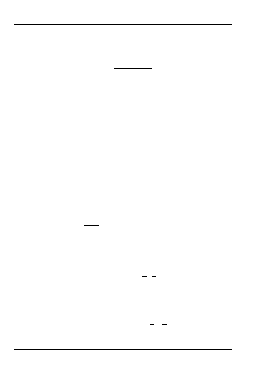
Code_Aster
®
Version
7.3
Titrate:
Law of behavior CAM-CLAY
Date:
03/02/05
Author (S):
J. EL GHARIB, G. DEBRUYNE
Key:
R7.01.14-B
Page
:
28/34
Manual of Reference
R7.01 booklet: Modelings for the Civil Engineering and the géomatériaux ones
HT-66/05/002/A
One poses
(
)
[
]
+
-
=
Cr
Cr
Cr
kP
M
P
P
kP
M
C
2
2
2
1
2
,
éq 5.3.2-12
[
]
+
=
Cr
Cr
kP
M
kP
M
has
2
2
2
1
2
éq 5.3.2-13
One has then:
+
=
C
P
has
P
Cr
éq 5.3.2-14
By replacing the expression of
Cr
P
in
[éq 5.3.2-7], one finds:
(
)
(
)
[
]
(
) (
) (
)
[
]
Cr
Cr
Cr
p
p
Cr
P
P
P
P
has
C
P
P
PP
H
B
km
H
P
P
has
C
P
M
P
P
P
M
2
2
4
1
.
2
2
2
4
2
2
-
+
+
-
-
-
-
+
-
=
éq 5.3.2-15
By gathering the terms in
and those in
P
, one finds:
P
E
F
=
éq 5.3.2-16
with,
(
)
[
]
(
)
(
)
[
]
Cr
Cr
Cr
p
Cr
p
P
P
aP
P
P
P
H
B
km
P
amndt
P
M
P
P
M
H
F
2
2
4
2
2
2
1
2
4
2
2
2
-
+
-
-
-
+
-
=
éq
5.3.2-17
(
)
Cr
p
p
P
P
P
H
bckM
H
P
cm
E
2
4
2
1
2
4
2
-
+
+
=
éq
5.3.2-18
The expression of
p
v
thus becomes:
(
)
P
P
P
E
F
E
F
C
has
M
Cr
p
v
-
+
-
-
=
2
2
éq 5.3.2-19
from where the expression of
v
according to
P
:
v
G
P
K
P
0
=
éq 5.3.2-20
(
)
-
+
-
-
+
=
Cr
P
P
E
F
C
E
F
has
P
K
M
G
0
2
2
1
éq 5.3.2-21

Code_Aster
®
Version
7.3
Titrate:
Law of behavior CAM-CLAY
Date:
03/02/05
Author (S):
J. EL GHARIB, G. DEBRUYNE
Key:
R7.01.14-B
Page
:
29/34
Manual of Reference
R7.01 booklet: Modelings for the Civil Engineering and the géomatériaux ones
HT-66/05/002/A
Calculus of the variation of deviatoric deformation:
ij
p
ij
PS
E
F
S
3
3
~
~
=
=
=
éq 5.3.2-22
One thus has finally:
P
F
ij
ij
=
éq 5.3.2-23
with
D
P
K
G
S
E
F
F
1
3
3
0
-
=
éq
5.3.2-24
5.3.3 Operator
tangent
The tangent operator connects the variation of total stress to the variation of total deflection. Being
given that the increment of the total deflection under loading deviatoric is written:
Mn
klmn
ij
kl
p
ijkl
ij
D
S
S
With
H
B
C
1
)
)
(
)
(
(
+
+
-
=
,
éq
5.3.3-1
with:
-
-
-
-
-
-
=
1
0
0
0
0
0
0
1
0
0
0
0
0
0
1
0
0
0
0
0
0
3
/
2
3
/
1
3
/
1
0
0
0
3
/
1
3
/
2
3
/
1
0
0
0
3
/
1
3
/
1
3
/
2
1
D
éq
5.3.3-2
projection in space deviatoric,
and that under spherical loading one a:
kl
kl
ij
ij
D
F
2
=
éq
5.3.3-3
with:
-
-
-
=
0
0
0
3
/
1
3
/
1
3
/
1
2
D
éq
5.3.3-4
hydrostatic projection, one has then:
kl
ijkl
ij
With
=
éq
5.3.3-5

Code_Aster
®
Version
7.3
Titrate:
Law of behavior CAM-CLAY
Date:
03/02/05
Author (S):
J. EL GHARIB, G. DEBRUYNE
Key:
R7.01.14-B
Page
:
30/34
Manual of Reference
R7.01 booklet: Modelings for the Civil Engineering and the géomatériaux ones
HT-66/05/002/A
with:
1
2
1
)
)
(
)
(
(
-
+
+
+
-
=
kl
ij
mnkl
ij
Mn
p
ijmn
ijkl
D
F
D
S
S
With
H
B
C
With
éq
5.3.3-6
the discretized tangent operator.
5.3.4 Tangent operator at the critical point
If the point of load is at the critical point
(
)
Cr
P
P
=
, the general expression of the tangent operator is not
more valid. This appears in particular by divide by 0 (see the equations of [§ 5.3.1]). One
detail in what follows the coherent tangent operator to the critical point while passing as for the case
General by the partly deviatoric and partly hydrostatic decomposition.
5.3.4.1 Processing of the deviatoric part
Let us recall that to the critical point, the expressions of the plastic multiplier
and of its derivation
are written in the following way:
µ
6
/
1
-
=
Q
Q
E
and
2
6
6
Q
Q
Q
Q
Q
E
E
µ
µ
-
=
éq
5.3.4.1-1
with,
E
E
E
E
Q
S
S
Q
2
3
=
and
Q
S
S
Q
2
3
=
éq
5.3.4.1-2
from where the expression of
:
-
=
3
2
3
6
1
Q
S
S
Q
Q
Q
S
S
E
E
E
E
µ
éq
5.3.4.1-1
Let us point out in the same way the expression of
S
:
(
)
ij
ij
ij
ij
S
S
S
µ
-
-
=
3
3
~
2
While replacing
and
by their expressions, one can write:
ij
E
ij
kl
kl
E
ij
E
E
kl
E
kl
ij
ij
S
Q
Q
S
S
S
Q
Q
S
Q
Q
S
S
S
µ
-
-
+
-
=
1
2
3
2
3
~
2
3
éq
5.3.4.1-2
kl
E
ij
E
kl
ijkl
ij
kl
E
ijkl
ijkl
E
ijkl
kl
Q
Q
S
S
S
S
Q
Q
Q
Q
S
µ
~
.
2
3
2
.
2
3
3
-
=
-
-
+
éq
5.3.4.1-5
or in tensorial writing:
µ
~
2
3
2
2
3
4
3
4
4
4 3
4
4 2
1
4
4
4
3
4
4
4
2
1
H
E
E
D
G
E
D
E
Q
Q
S
S
I
S
S
Q
Q
I
Q
Q
S
-
=
-
éq
5.3.4.1-6

Code_Aster
®
Version
7.3
Titrate:
Law of behavior CAM-CLAY
Date:
03/02/05
Author (S):
J. EL GHARIB, G. DEBRUYNE
Key:
R7.01.14-B
Page
:
31/34
Manual of Reference
R7.01 booklet: Modelings for the Civil Engineering and the géomatériaux ones
HT-66/05/002/A
Like
S
does not depend on
v
, one can confuse
~
with
.
By using the tensor of projection in the space of the deviatoric stresses
1
D
[éq 5.3.3-2], one
can write:
µ
.
2
.
.
1
1
-
=
H
G
D
éq
5.3.4.1-7
5.3.4.2 Processing of the hydrostatic part
In tensorial writing, one with the following relation:
v
D
P
K
P
I
0
=
.
éq 5.3.4.2-1
according to the equation [éq 5.3.2-2] with
0
=
p
v
at the critical point.
Like
P
does not depend on
~
then one can confuse
v
with
.
P
K
P
I
D
0
=
éq
5.3.4.2-2
By using the tensor of projection in the space of the hydrostatic stresses
2
D
[éq 5.3.3-4], one
can write:
2
0
D
P
K
I
D
=
éq
5.3.4.2-3
5.3.4.3 Tangent operator
By combining the contributions of the two parts deviatoric and hydrostatic, one finds the writing of
the tangent operator who connects the variation of the total stress to the variation of the total deflection to
not criticizes:
µ
.
2
.
.
2
0
1
1
+
=
-
D
P
K
I
H
G
D
D
or
kl
ijkl
ij
With
=
éq
5.3.4.3-1
with
1
2
0
1
1
2
.
.
-
-
+
=
D
P
K
I
H
G
D
With
D
ijkl
µ
éq
5.3.4.3-2

Code_Aster
®
Version
7.3
Titrate:
Law of behavior CAM-CLAY
Date:
03/02/05
Author (S):
J. EL GHARIB, G. DEBRUYNE
Key:
R7.01.14-B
Page
:
32/34
Manual of Reference
R7.01 booklet: Modelings for the Civil Engineering and the géomatériaux ones
HT-66/05/002/A
6
Examples of implementation of the model
6.1
Initialization of calculation
In the model
CAM_CLAY
, the non-linear elastic law reveals a hydrostatic stress
for a null voluminal deformation [éq 3.3-4]. One thus needs at the beginning for calculations to initialize
hydrostatic stress with a strictly positive value. With this intention, one can proceed of two
different ways:
To carry out a linear elastic design by affecting boundary conditions such as the field of
forced in the structure is a uniform hydrostatic compression equal to pressure AP
data in
DEFI_MATERIAU
. Pressure AP corresponds to the initial index of the vacuums and is
generally equalizes with the atmospheric pressure (the latter is given positively to be
coherent with conventions of the civil engineering). One extracts from this calculation the stress field with
points of Gauss. This stress field is regarded as the initial state of the stress
hydrostatic necessary to the law
CAM_CLAY
in calculation
STAT_NON_LINE
using the model
CAM_CLAY
.
To use the operator
CREA_CHAMP
to create with the operation
“AFFE”
a stress field
hydrostatic to the points of Gauss of value AP, the stress in this case is given of sign
negative (convention Aster for compressions) and constitutes the initial state in
STAT_NON_LINE
according to.
Numerical results for triaxial compression tests.
The following figures show triaxial ways of loading with evolutions of
axial deformation according to the diverter
Q
. They result from numerical calculations carried out
with model CAM-CLAY established in Code_Aster. These test were carried out by using one
modeling of the type
KIT_HM
in not drained condition (this condition allows us easily
to charge in a purely deviatoric way, the hydrostatic part of the loading being taken again by
pressure of water). The shapes of the curves obtained numerically with Code_Aster are very with
fact comparable with the diagrammatic curves presented in the paper of Charlez [bib2].
In the first test, the material is normally consolidated, i.e. hydrostatic pressure
of departure is equal to the pressure of consolidation (in this case
5
10
.
6
AP). Work hardening (positive)
start at the beginning of the deviatoric phase, without preliminary elastic phase. Hardening
continue to a bearing of perfect plasticity when the critical point is reached (Q=MP).
As for the three other tests, the deviatoric phase starts for a value of the stress
effective average lower than the pressure of consolidation, the material is of this surconsolidé fact.
If
P
is higher than
Cr
P
equalize with
5
10
.
3
AP, the specific point of the loading cross
surface of load before the critical line. There will be thus three specific phases: a phase
rubber band, a contracting plastic phase then a perfect plastic phase.
If
Cr
P
P
=
, the behavior is plastic perfect right after the elastic phase.
In the case where
P
is lower than
Cr
P
, the point representative of the loading cuts the critical line
before the surface of load which it reaches during a purely elastic way. In this
configuration, the behavior is lenitive and dilating and locked energy decreases. The point
representative of the loading joined then the critical state where the material will enter in perfect plasticity.
The Cam_Clay behavior cannot produce a behavior continuement contractor/dilating.
not representative of the loading is obliged to pass by the critical state where the whole of the parameters
of work hardening (plastic voluminal deformation, critical pressure, locked energy) become
stationary [bib2].
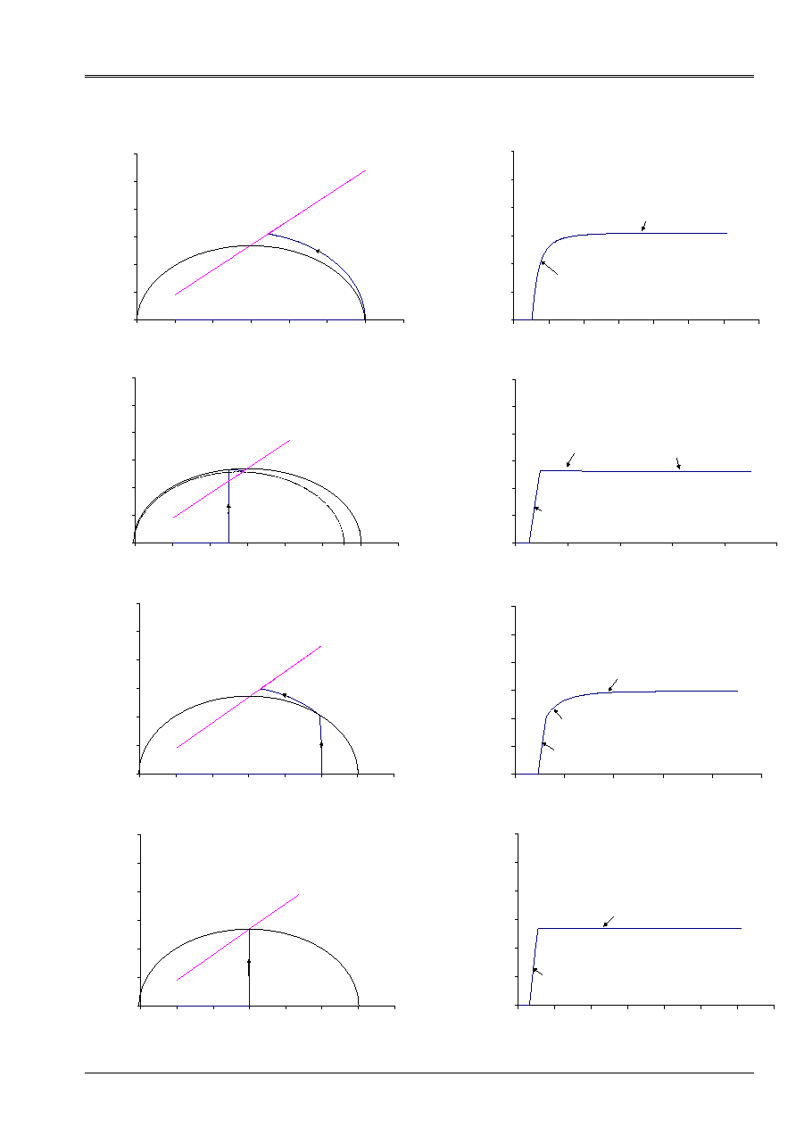
Code_Aster
®
Version
7.3
Titrate:
Law of behavior CAM-CLAY
Date:
03/02/05
Author (S):
J. EL GHARIB, G. DEBRUYNE
Key:
R7.01.14-B
Page
:
33/34
Manual of Reference
R7.01 booklet: Modelings for the Civil Engineering and the géomatériaux ones
HT-66/05/002/A
0,00E+00
1,00E+05
2,00E+05
3,00E+05
4,00E+05
5,00E+05
6,00E+05
0, E+00
5, E-02
1, E-01
2, E-01
2, E-01
3, E-01
eps1
Q (
AP
)
rubber band
hardening
critical state
0,00E+00
1,00E+05
2,00E+05
3,00E+05
4,00E+05
5,00E+05
6,00E+05
0
100000 200000 300000 400000 500000 600000 700000
P (AP)
Q (AP)
Q=MP
0,00E+00
1,00E+05
2,00E+05
3,00E+05
4,00E+05
5,00E+05
6,00E+05
0, E+00 5, E-02 1, E-01 2, E-01 2, E-01 3, E-01 3, E-01 4, E-01
eps1
Q (AP
)
rubber band
critical state
0,00E+00
1,00E+05
2,00E+05
3,00E+05
4,00E+05
5,00E+05
6,00E+05
0
100000 200000 300000 400000 500000 600000 700000
P (AP)
Q (AP)
Q=MP
0,00E+00
1,00E+05
2,00E+05
3,00E+05
4,00E+05
5,00E+05
6,00E+05
0, E+00
5, E-02
1, E-01
2, E-01
2, E-01
3, E-01
eps1
Q (AP)
rubber band
radoucissement
critical state
0,00E+00
1,00E+05
2,00E+05
3,00E+05
4,00E+05
5,00E+05
6,00E+05
0
100000 200000 300000 400000 500000 600000 700000
P (AP)
Q (AP)
0,00E+00
1,00E+05
2,00E+05
3,00E+05
4,00E+05
5,00E+05
6,00E+05
0, E+00 5, E-02
1, E-01
2, E-01
2, E-01
3, E-01
3, E-01 4, E-01
eps1
Q (
P
has)
hardening
Critical State
0,00E+00
1,00E+05
2,00E+05
3,00E+05
4,00E+05
5,00E+05
6,00E+05
0
100000 200000 300000 400000 500000 600000 700000
P (AP)
Q (AP
)
Q=MP

Code_Aster
®
Version
7.3
Titrate:
Law of behavior CAM-CLAY
Date:
03/02/05
Author (S):
J. EL GHARIB, G. DEBRUYNE
Key:
R7.01.14-B
Page
:
34/34
Manual of Reference
R7.01 booklet: Modelings for the Civil Engineering and the géomatériaux ones
HT-66/05/002/A
7 Bibliography
[1]
I.B BURLAND, K.H. ROSCOE: One the generalized stress strain behavior off wet clay,
Engineering plasticity Cambridge Heyman-Leckie, 1968.
[2]
PH. A. CHARLEZ (Total Report/ratio): Example of model poroplastic: the model of
Camwood-Clay.
[3]
NR. TARDIEU, I. VAUTIER, E. LORENTZ
: Quasi-static nonlinear algorithm.
Reference material Aster [R5.03.01].
[4]
J. LEMAITRE, J.L. CHABOCHE: mechanics of solid materials, Dunod 1985