
Code_Aster
®
Version
7.4
Titrate:
Multiaxial criteria of priming in fatigue to great number of cycle
Date
:
01/09/05
Author (S):
J. ANGLES
Key
:
R7.04.04-A
Page
:
1/36
Manual of Reference
R7.04 booklet: Evaluation of the damage
HT-66/05/002/A
Organization (S):
EDF-R & D/AMA
Manual of Reference
R7.04 booklet: Evaluation of the damage
Document: R7.04.04
Multiaxial criteria of priming in fatigue to large
numbers of cycle: models of DANG VAN and
MATAKE
Summary:
In this note we propose a formulation of the criteria of MATAKE and DANG VAN within the framework of
office plurality of damage under periodic and nonperiodic multiaxial loading.
The first part of this document is devoted to the criteria of MATAKE and DANG VAN adapted to
periodic multiaxial loadings. In this part after having approached the concepts of endurance and office plurality
of damage and the general form of the criteria of fatigue, we describe the two models of DANG VAN and
MATAKE (Plane criticizes) designed to carry out calculations of office plurality of damage under multiaxial loading.
One details there the definition of the various plans of shearing associated with the points of Gauss or the nodes, thus
that the definition of an amplitude of loading through the circle circumscribed with the way of the loading in
plan of shearing. Finally the criteria available in Code_Aster are presented.
In the second part we propose a formulation of the criteria of MATAKE and DANG VAN in
tally of the office plurality of damage under nonperiodic multiaxial loading. To define a cycle in the case
variable amplitude, we reduce the history of the loading to a unidimensional function of time in
projecting the point of the vector shearing on an axis, and we use a method of counting of cycles. Here
we choose method RAINFLOW. Criteria of MATAKE and DANG VAN adapted to the office plurality of
damage under nonperiodic loading are established in Code_Aster.

Code_Aster
®
Version
7.4
Titrate:
Multiaxial criteria of priming in fatigue to great number of cycle
Date
:
01/09/05
Author (S):
J. ANGLES
Key
:
R7.04.04-A
Page
:
2/36
Manual of Reference
R7.04 booklet: Evaluation of the damage
HT-66/05/002/A
Count
matters

Code_Aster
®
Version
7.4
Titrate:
Multiaxial criteria of priming in fatigue to great number of cycle
Date
:
01/09/05
Author (S):
J. ANGLES
Key
:
R7.04.04-A
Page
:
3/36
Manual of Reference
R7.04 booklet: Evaluation of the damage
HT-66/05/002/A
1 Introduction
The models of endurance in fatigue multiaxial under periodic loading are models of
following type:
B
average
VAR
has
amplitude
VAR
<
+
_
_
,
where
B
is the threshold of endurance in simple shearing, and has a positive constant without dimension.
amplitude
VAR _
is a certain definition of the amplitude (half of the variation) of the cycle of
loading and
average
VAR _
is a variable in connection with the stress (or sometimes
deformation) or stresses (or sometimes deformations) average. The models are distinguished
by definitions different from
amplitude
VAR _
and
average
VAR _
.
To pass from the endurance to the office plurality of the damage, a definite equivalent stress is introduced
by:
average
VAR
has
amplitude
VAR
eq
_
_
+
=
.
This equivalent stress gives us a unit damage on the curve of fatigue. Like
second member of the inequation
B
corresponds to the threshold in shearing, one needs a curve of fatigue in
shearing. But the curves of fatigue in shearing are rare since difficult to obtain, one
thus try to use the curves of fatigue in traction alternate compression. For that it is necessary
to about multiply the equivalent stress by a corrective coefficient
3
.
The macroscopic models of MATAKE (plane criticizes) and macro microcomputer of DANG VAN are described.
It is shown that under certain assumptions the model of DANG VAN is similar to the model
macroscopic of MATAKE. The only difference lies in the variable
average
VAR _
: DANG
VAN uses the hydrostatic pressure, while MATAKE employs the normal stress on the plan
of maximum amplitude of shearing.
After having defined the plan of shearing, we express the shear stress in this plan.
The plans of shearing are then explored according to a method described in the reference [bib4] which
consist in cutting out the surface of a sphere of pieces of equal sizes.
The normal vectors being known we then determine for each plan the points which are them
more distant from/to each other. Among those we find the two points which are most distant
one of the other. That being made we use, if necessary, the method of the circle passing by three
points in order to obtain the circle circumscribed with the way of loading.
In the first part of this document we present the models of endurance in fatigue
multiaxial under loading periodicals As well as the concept of office plurality of damage. The passage of
the endurance with the office plurality of damage is also approached.
In the second part the criteria of MATAKE and DANG VAN are then presented under
aspects limits endurance and office plurality of damage under periodic loading.
The third part is devoted to the definition of the plan of shearing, of the expression of the stresses
of shearing in this plan and finally, with the manner of exploring the plans of shearing.
The fourth part is dedicated to the determination of the circle circumscribed with the way of shearing in
plan of the same name. Finally we describe the criteria and the sizes which are introduced into
Code_Aster.
After having extended the models of MATAKE and DANG VAN to the office plurality of damage under loading
periodical, we present the adaptation of these models at the office plurality of damage under loading
not periodical. Thus, the fifth part is devoted to the definition of the equivalent stress
elementary.
The sixth part deals with the manner of selecting the axis (or the two axes) on which is
projected the history of the cission.
The seventh part is dedicated to projection itself of the point of the vector cission on this
center or these two axes. Lastly, concerning the criteria of MATAKE and DANG VAN formulated in office plurality of
damage under nonperiodic loading, we describe the sizes which are introduced into
Code_Aster.

Code_Aster
®
Version
7.4
Titrate:
Multiaxial criteria of priming in fatigue to great number of cycle
Date
:
01/09/05
Author (S):
J. ANGLES
Key
:
R7.04.04-A
Page
:
4/36
Manual of Reference
R7.04 booklet: Evaluation of the damage
HT-66/05/002/A
2 Preliminaries
In this part we treat the concepts of limit of endurance and office plurality of damage. Us
also let us present the general form of the criteria of fatigue.
2.1
Limit of endurance and office plurality of damage, uniaxial case
In the uniaxial case the rigorous definition of a threshold of endurance it is the half-amplitude (half
variation) of loading defined in stress in lower part of which the lifespan is infinite.
However, as in practice the lifespan cannot never be infinite, one defines limits
of endurance with 10
7
, 10
8
, etc cycles of loading. There is another way of seeing the things:
since in practice the infinite lifespan does not exist, one uses the concept of office plurality of damage.
The approach by the office plurality of damage consists in defining a limit in a number of cycles beyond
which the cumulated damage is equal to one. Thus limit with 10
7
wants to say that after 10
7
cycles it
cumulated damage is equal to 1.
2.2
Criterion of fatigue, multiaxial case
In the literature a certain number of criteria were proposed to define the threshold of endurance
under multiaxial cyclic loading. The general form of these criteria is:
B
average
VAR
has
amplitude
VAR
<
+
_
_
éq
2.2-1
where
B
is the threshold of endurance in simple shearing,
has
is a positive constant without dimension.
amplitude
VAR _
is a certain definition of the half-amplitude (half of the variation) of the cycle
and
average
VAR _
is a variable in connection with the stress (or sometimes deformation) or them
stresses (or sometimes deformations) average. Various models are characterized by
definitions different from
amplitude
VAR _
and
average
VAR _
.
To pass from the endurance to the office plurality of the damage, one can define a stress (or one
deformation) equivalent:
average
VAR
has
amplitude
VAR
eq
_
_
+
=
éq
2.2-2
This equivalent stress gives us a unit damage on the curve of fatigue. Like
second member of the inequation [éq 2.2-1] corresponds to the threshold in shearing, one needs a curve of
tire in shearing. But the curves of fatigue in shearing are rare since difficult with
to obtain, one thus tries to use the curves of fatigue in traction alternate compression. For that it
is necessary to be coherent at least for the level of the threshold of endurance i.e. to multiply
eq
by one
constant about
3
to be able to use the curve of fatigue in traction. The value
3
is
exact value for a criterion of the type Put, in experiments this coefficient is smaller than
3
.
2.3
Definition of an amplitude of loading in the multiaxial case
In Code_Aster, there are two definitions of amplitude of loading in the multiaxial case:
A: radius (half diameter) of the sphere circumscribed with the way of the loading;
B: half of the maximum of the distance between two unspecified points of the way.
It is clear that in the case of a loading being defined on a sphere A and B give the same one
amplitude. On the other hand, if one takes a way (two-dimensional) in the form of a triangle equilateral of
dimensioned
L
, definition A gives us
3
L
, while the definition B gives us
2
/
L
. To work
within a conservative framework we take as definition of the amplitude (half-variation) of a way of
loading the radius of the sphere (or rings for the case 2D) circumscribed.
Code_Aster
®
Version
7.4
Titrate:
Multiaxial criteria of priming in fatigue to great number of cycle
Date
:
01/09/05
Author (S):
J. ANGLES
Key
:
R7.04.04-A
Page
:
5/36
Manual of Reference
R7.04 booklet: Evaluation of the damage
HT-66/05/002/A
2.4
Definition of the plan of shearing
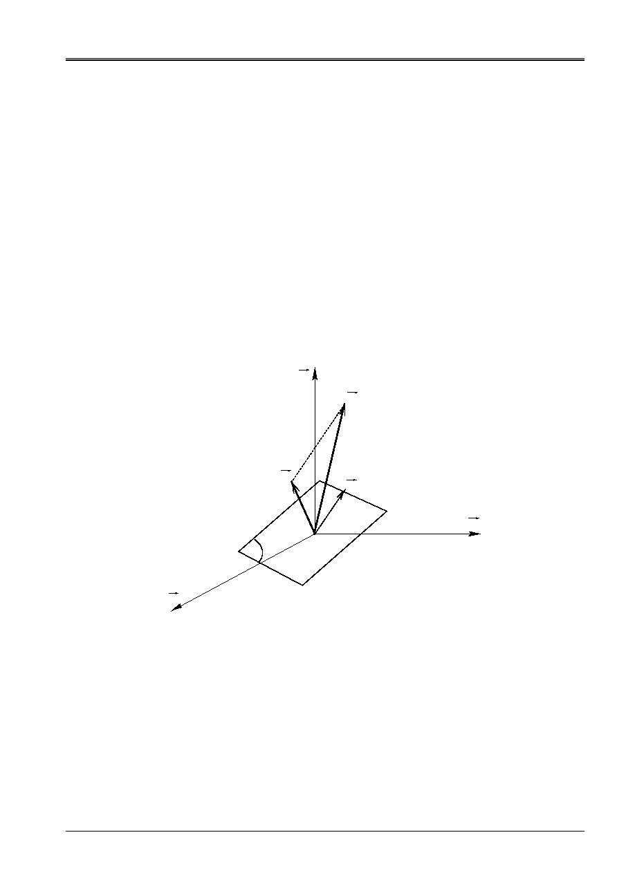
In a point M of a continuous medium we express the tensor of the stresses
in a reference mark
orthonormé
)
,
,
,
(
Z
y
X
O
. With the unit normal
N
components
)
,
,
(
Z
y
X
N
N
N
in the reference mark
orthonormé, we associate the vector forced
N
F
.
=
components
)
,
,
(
Z
y
X
F
F
F
. It
vector
F
can break up into a normal vector with
N
and a scalar carried by
N
, that is to say:
+
=
N
F
NR
éq 2.4-1
where
NR
represent the normal stress and the vector
the shear stress. In the reference mark
)
,
,
,
(
Z
y
X
O
, components of the vector
are noted:
)
,
,
(
Z
y
X
. The vector
results
directly of [éq 2.4-1] and the normal stress:
.
.
;
.
N
N
F
F
N
F
-
=
=
where
of
NR
éq
2.4-2
N
F
Z
y
X
O
Appear 2.4-a: Representation of the vectors of stress
F
and of shear stress

Code_Aster
®
Version
7.4
Titrate:
Multiaxial criteria of priming in fatigue to great number of cycle
Date
:
01/09/05
Author (S):
J. ANGLES
Key
:
R7.04.04-A
Page
:
6/36
Manual of Reference
R7.04 booklet: Evaluation of the damage
HT-66/05/002/A
3
Model of MATAKE (plane criticizes) and model of DANG VAN
Here we clarify the criterion of MATAKE and DANG VAN at the same time from the limiting point of view
of endurance and the point of view of the office plurality of damage.
3.1
Criterion of MATAKE
In this type of criterion the calculation of the deformation and stress fields is made under the assumption
of elasticity, cf reference [bib1]. Like it was known as in chapter 2, in the multiaxial case the criterion
of endurance is generally written in the form:
B
average
VAR
has
amplitude
VAR
<
+
_
_
éq
3.1-1
Amplitude of loading: In the case of the criterion of MATAKE at each point of the structure (or
not Gauss for a calculation with the finite elements) to calculate
amplitude
VAR _
one proceeds of
following way:
·
for each plan of normal
N
one calculates the amplitude of shearing by determining the circle
circumscribed with the way of shearing in this plan;
·
the normal is sought
*
N
for which the amplitude is maximum. This amplitude is
indicated by
*)
(N
.
Mean stress: For the calculation of
average
VAR
_
one proceeds in the following way:
·
within normal
*
N
one calculates on a cycle the indicated maximum normal stress
by
*)
(
max
N
NR
.
The criterion of endurance is written:
B
NR
has
+
*)
(
2
*)
(
max
N
N
,
where
has
and
B
are two positive constants and
B
represent the limit of endurance in simple shearing.
Identification of the constants: to determine the constants
has
and
B
two tests should be used
simple. Two possibilities exist:
A pure shear test plus an alternate tensile test compression. In this case constants
are given by:
0
=
B
2
2
0
0
0
D
D
has
-
=
, where
0
represent the limit of endurance in
alternated pure shearing and
0
D
limit of endurance in alternate pure traction and compression.
Two tensile tests compression, alternated and the other not. The constants are given by:
(
)
(
)
(
)
2
2
,
2
1
1
2
2
1
1
2
×
+
-
=
-
-
-
=
m
m
m
B
has
where
1
is the amplitude of loading for the alternate case and
2
for the case where the stress
average is nonnull.

Code_Aster
®
Version
7.4
Titrate:
Multiaxial criteria of priming in fatigue to great number of cycle
Date
:
01/09/05
Author (S):
J. ANGLES
Key
:
R7.04.04-A
Page
:
7/36
Manual of Reference
R7.04 booklet: Evaluation of the damage
HT-66/05/002/A
3.2
Criterion of DANG VAN
It is supposed that the material remains overall elastic while it is plasticized locally.
The interesting physical assumption of the model is that the material adapts locally (it becomes
rubber band after having passed by plasticity) below the limit of endurance, which corresponds to
nonthe initiation of fissure. Above the limit of endurance there is locally accommodation
plastic thus initiation of fissure.
The basic assumptions of the microcomputer-macro interaction, Flax-Taylor, make it possible to write:
)
(
2
)
(
)
(
)
(
)
(
T
T
T
T
T
p
ij
ij
ij
ij
Loc
ij
µ
-
=
+
=
One indicates the local stress by
)
(T
Loc
ij
, the total stress by
)
(T
ij
, the residual stress
local by
()
T
ij
and by
)
(T
p
ij
local plastic deformation. As soon as there is adaptation the deformation
figure local becomes constant and thus the local residual stress also.
Criterion of plasticity:
In a point of the continuous medium (where there is a distribution of the crystallographic directions random of
grains), it is supposed that there is only one grain which is plasticized and this, following only one system of
slip. This system of slip will be that which will be most favorably directed, i.e., it
grain in which the greatest scission (the projection of the vector shearing will occur on one
direction given). The slip is done in the plans of normal
)
,
,
(
3
2
1
N
N
N
=
N
and direction of
slip is defined by the vector
)
,
,
(
3
2
1
m
m
m
=
m
. Two vectors
N
and
m
are
orthogonal.
The law of Schmid says that so that there is no irreversible slip (plastic deformation) it is necessary
that the scission, does not exceed a certain threshold, that is to say:
0
)
(
)
,
,
(
-
T
T
Loc
y
Loc
m
N
N
m
éq
3.2-1
where
)
(
2
1
)
(
J
I
J
I
ij
loc
ij
ij
Loc
m
N
N
m
has
and
has
T
+
=
=
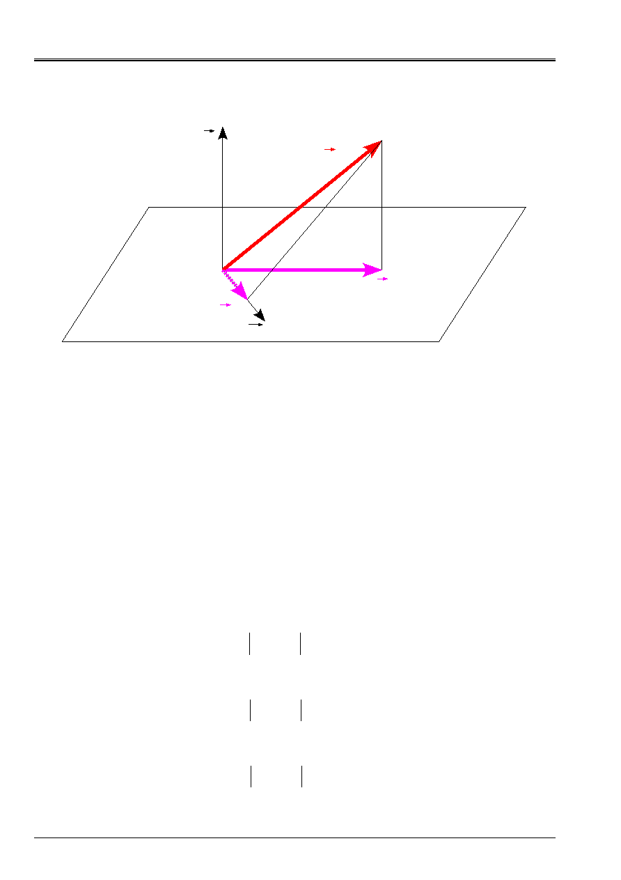
The drawing of [Figure 3.2-a] shows that the maximum value of
Loc
, indicated by
Loc
max
, is obtained
by the orthogonal projection of
J
Loc
ij
Loc
N
F
=
within normal
N
. The relation [éq 3.2-1] must
in particular to be checked if one replaces
Loc
by its raising
Loc
max
, the aforementioned is written
then:
0
)
(
)
,
(
max
-
T
T
Loc
y
Loc
N
N
éq
3.2-2
where
)
(T
Loc
y
is the threshold of the microscopic or local scission.
)
(T
Loc
y
depends on the variables
of work hardening.
Code_Aster
®
Version
7.4
Titrate:
Multiaxial criteria of priming in fatigue to great number of cycle
Date
:
01/09/05
Author (S):
J. ANGLES
Key
:
R7.04.04-A
Page
:
8/36
Manual of Reference
R7.04 booklet: Evaluation of the damage
HT-66/05/002/A
N
m
Loc
max
Loc
F
Loc
Appear 3.2-a: Projection of
Loc
F
within normal
N
One chooses a microscopic work hardening of the linear isotropic type. That makes it possible to show the existence
of a field of adaptation [bib2], [bib3].
In the state adapted by analogy with the formula:
*
)
(
)
(
ij
ij
Loc
ij
T
T
+
=
one has, if one places oneself in the plan
)
,
(m
N
in such a way that the scission is maximum, the formula
following:
)
(
)
,
(
)
,
(
max
N
N
N
+
=
T
T
Loc
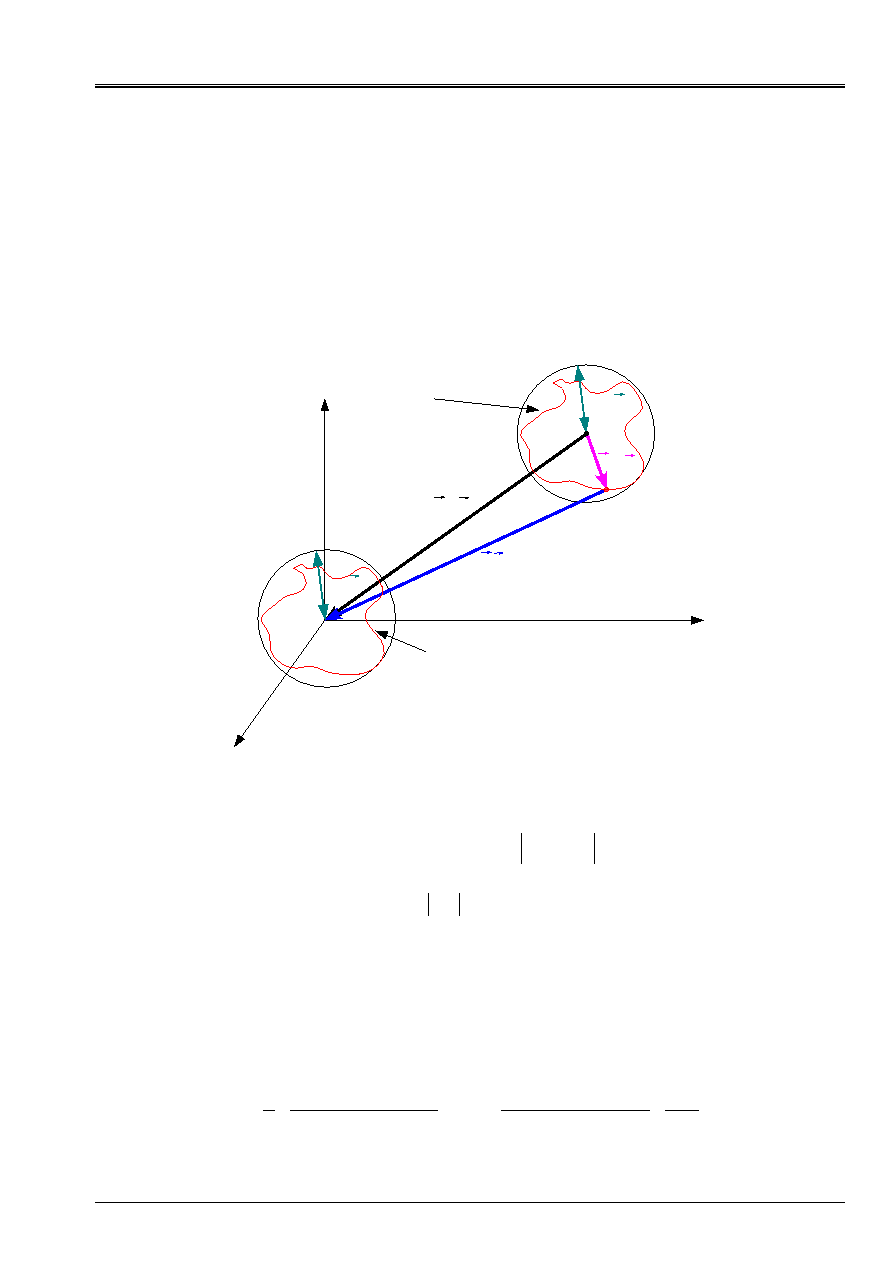
where
)
,
(T
N
is the vector macroscopic shearing defined in [the Figure 3.2-b] and where
)
(N
is it
vector microscopic residual shearing (independent of time since we are with the state
adapted).
Criterion of fatigue
Introduction of the maximum pressure: DANG VAN uses in the place of the normal stress on one
plan, as that is done in model MATAKE, the maximum hydrostatic pressure on a cycle.
The criterion is thus written:
(
)
B
P
has
T
MAX
Loc
Loc
T
+
max
max
,
)
,
(N
N
As the hydrostatic pressures local and total are identical the criterion becomes:
(
)
B
P
has
T
MAX
Loc
T
+
max
max
,
)
,
(N
N
For a positive maximum pressure we have:
(
)
B
P
has
T
MAX
Loc
T
+
max
max
,
)
,
(N
N
Code_Aster
®
Version
7.4
Titrate:
Multiaxial criteria of priming in fatigue to great number of cycle
Date
:
01/09/05
Author (S):
J. ANGLES
Key
:
R7.04.04-A
Page
:
9/36
Manual of Reference
R7.04 booklet: Evaluation of the damage
HT-66/05/002/A
For an always negative pressure one can take
0
max
=
P
to remain conservative.
Assumption on
)
(N
In the radial case where the direction of maximum shearing is defined in advance one can calculate
exact way
)
(N
. In general case DANG VAN proposes the following method to do one
calculation simplified of
)
(N
. One gives for a plan
N
the macroscopic way of the vector shearing
defined previously. The vector residual shearing taking into account the preceding assumption is
defined by MO, where M is the center of the circle circumscribed with the way of the end of the vector shearing
in the plan of shearing.
0
M
P
(N, T
I
)
(N, T
I
)
Loc
max
(N)
Plan of
shearing
Macroscopic way
Microscopic way
(N)
Loc
max
(N)
Loc
max
Appear 3.2-b: Ways macro microcomputer/in the plan of shearing
Final formulation: taking into account the two formulas:
(
)
B
P
has
T
MAX
T
T
Loc
T
Loc
+
+
=
max
max
,
max
)
,
(
)
(
)
,
(
)
,
(
N
N
N
N
N
and
one finds oneself with
()
B
P
has
MAX
T
+
max
,
MP
N
where
P
is a point running of the way of shearing in the plan of normal
N
.
Identification of the constants: to determine the constants
has
and
B
two tests should be used
simple. Two possibilities exist:
1) A pure shear test plus a tensile test alternate compression. In it
cases the constants are given by:
)
3
/
/(
)
2
/
(
0
0
0
0
D
D
has
B
-
=
=
.
2) Two tensile tests compression, alternated and the other not. The constants are
data by:
(
)
(
)
(
)
2
2
2
2
3
1
1
2
2
1
1
2
×
+
-
=
-
-
-
×
=
m
m
m
B
has
.
with
1
the amplitude of loading for the alternate case and
2
for the case where the stress
average is nonnull.

Code_Aster
®
Version
7.4
Titrate:
Multiaxial criteria of priming in fatigue to great number of cycle
Date
:
01/09/05
Author (S):
J. ANGLES
Key
:
R7.04.04-A
Page
:
10/36
Manual of Reference
R7.04 booklet: Evaluation of the damage
HT-66/05/002/A
3.3
MATAKE and DANG VAN modified for the office plurality of damage
The models of MATAKE and DANG VAN were proposed initially for the study of the limit
of endurance. As the infinite lifespan does not exist one uses limits of endurance with, 10
6
, 10
7
,
10
N
cycles of loading. Thus the initial criteria of MATAKE and DANG VAN are presented like
criteria of going beyond of a threshold and do not give an office plurality of damage. The use,
in particular criterion of DANG VAN, in the car industries is suitable since the objective
sought is nonthe going beyond of a threshold of endurance contrary to the problems of EDF where
one wishes to follow the damage.
Thus we use for the office plurality of damage an equivalent stress of MATAKE or DANG
VAN defined by:
()
()
()
.
,
*
*
2
max
,
max
aP
MAX
N
NR
has
N
T
eq
eq
+
=
+
=
MP
N
VAN
DANG
MATAKE
The taking into account of the surface treatment east summarized with the taking into account of the harmful effect of
pre-work hardening over the lifespan in controlled deformation [bib5]. In the models of MATAKE and
DANG VAN the effect of pre-work hardening is taken into account by multiplying the half-amplitude of stress
of shearing by a corrective coefficient higher than the unit, noted
p
C
:
()
()
()
.
,
*
*
2
max
,
max
aP
MAX
C
N
NR
has
N
C
T
p
eq
p
eq
+
=
+
=
MP
N
VAN
DANG
MATAKE
These equivalent stresses are to be used on a curve of fatigue in shearing. For the use
on a curve of fatigue in traction compression it is necessary to multiply these equivalent stresses by one
corrective coefficient, noted here
:
()
()
()
.
,
*
*
2
max
,
max
+
=
+
=
aP
MAX
C
N
NR
has
N
C
T
p
eq
p
eq
MP
N
VAN
DANG
MATAKE
Code_Aster
®
Version
7.4
Titrate:
Multiaxial criteria of priming in fatigue to great number of cycle
Date
:
01/09/05
Author (S):
J. ANGLES
Key
:
R7.04.04-A
Page
:
11/36
Manual of Reference
R7.04 booklet: Evaluation of the damage
HT-66/05/002/A
4
Calculation of the plan of maximum shearing
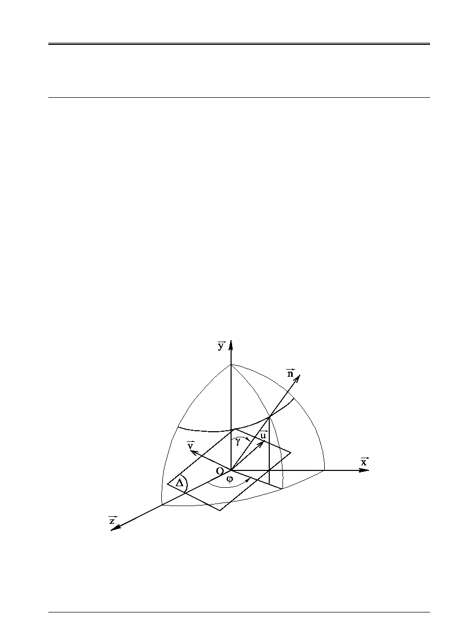
We use here the definition of the plan of shearing introduced in the paragraph [§2.4]. Practically,
for us the point M of the continuous medium will be a point of Gauss.
4.1
Expression of shear stresses in the plan
For reasons of symmetry we vary the unit normal
N
according to a half-sphere with aid
angles
and
, cf [Figure 4.1-a].
In the reference mark
)
,
,
,
(
Z
y
X
O
, the unit normal vector
N
is defined by:
cos
sin
sin
cos
sin
=
=
=
Z
y
X
N
N
N
. éq
4.1-1
We introduce a new reference mark
)
,
,
,
(
N
v
U
O
where
N
is perpendicular to the plan of shearing
and where
U
and
v
are in this plan, cf [Figure 4.1-a]. In the reference mark
)
,
,
,
(
Z
y
X
O
vectors
unit
U
and
v
are respectively defined by:
0
cos
sin
=
=
-
=
Z
y
X
U
U
U
,
éq
4.1-2
sin
sin
cos
cos
cos
=
-
=
-
=
Z
y
X
v
v
v
.
éq
4.1-3
Appear 4.1-a: Identification of the normal
N
in a plan by the angles
and
Code_Aster
®
Version
7.4
Titrate:
Multiaxial criteria of priming in fatigue to great number of cycle
Date
:
01/09/05
Author (S):
J. ANGLES
Key
:
R7.04.04-A
Page
:
12/36
Manual of Reference
R7.04 booklet: Evaluation of the damage
HT-66/05/002/A
In the plan
, components
U
and
v
vector
representing the shear stress
are obtained by the relations:
Z
Z
y
y
X
X
U
U
U
U
+
+
=
=
U
,
éq
4.1-4
Z
Z
y
y
X
X
v
v
v
v
+
+
=
=
v
.
éq
4.1-5
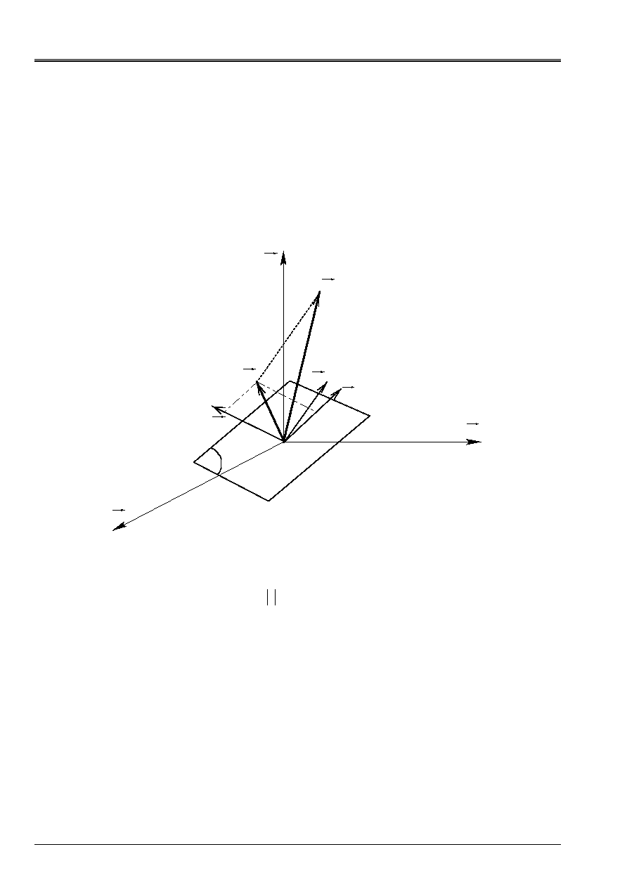
On [Figure 4.1-b], we represented shear stresses in the plan
as well as
identify
)
,
,
,
(
N
v
U
O
.
v
F
N
U
Z
X
y
O
Appear 4.1-b: Representation of the vector stress shear
in the plan
Now our problems are to determine for each point of Gauss or each node of one
mesh the plan of normal
N
such as
that is to say maximum. With this intention we vary the normal
unit
N
.
4.2
Browsing of the plans of shearing
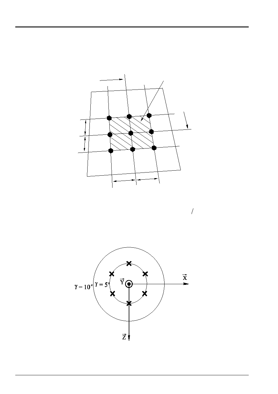
The method that we present here results from the reference [bib4]. Its principle is as follows.
As indicated in the paragraph [§4.1], for reasons of symmetry we vary the normal
unit
N
according to a half-sphere using the angles
and
, cf [Figure 4.1-a]. The question which comes
immediately is which must be the pitch of variation of the angles
and
. Indeed, one should be found
optimum between the smoothness of browsing and a reasonable time calculating insofar as it is
necessary to make this operation at each point of Gauss of the mesh. The author of the reference [bib4]
propose to divide the surface of the half sphere into breakages of equal surfaces to the center of which
unit normal
N
is positioned, cf [Figure 4.2-a]. In practice surfaces are not strictly
equal but of the same order of magnitude.
The step value of variation of
,
is worth 10 degrees. The angle
vary according to a pitch
who is
function of the angle
. More
is weak or close to 180 degrees and more
must be large for
to preserve a surface of about constant breakage. It is in the vicinity of
°
=
90
that
is more
small. [Table 4.2-1] the cutting summarizes which was retained.

Code_Aster
®
Version
7.4
Titrate:
Multiaxial criteria of priming in fatigue to great number of cycle
Date
:
01/09/05
Author (S):
J. ANGLES
Key
:
R7.04.04-A
Page
:
13/36
Manual of Reference
R7.04 booklet: Evaluation of the damage
HT-66/05/002/A
With this method the number of breakage thus the number of normal vectors to explore is equal to
209 for a half sphere.
X
Appear 4.2-a: Division of the surface of the half sphere in breakages
°
°
0
°
10
°
20
°
30
°
40
°
50
°
60
°
°
180
°
60
°
30
°
20
°
15
°
857
,
12
°
25
,
11
A number of breakages
1
3
6
9
12
14
16
°
°
70
°
80
°
90
°
100
°
110
°
120
°
130
°
°
588
,
10
°
10
°
10
°
10
°
588
,
10
°
25
,
11
°
857
,
12
A number of breakages
17
18
18
18
17
16
14
°
°
140
°
150
°
160
°
170
°
180
°
°
15
°
20
°
30
°
60
°
180
A number of breakages
12
9
6
3
1
Table 4.2-1: Numbers of breakage according to
and of
Code_Aster
®
Version
7.4
Titrate:
Multiaxial criteria of priming in fatigue to great number of cycle
Date
:
01/09/05
Author (S):
J. ANGLES
Key
:
R7.04.04-A
Page
:
14/36
Manual of Reference
R7.04 booklet: Evaluation of the damage
HT-66/05/002/A
In order to determine the normal vector
N
who will give the plan of maximum shearing except for the degree,
the author recommends to resort to two additional successive refinings. The first consists with
to explore eight new breakages around the initial normal vector, like illustrates it it [Figure 4.2-b].
max
Facet F
m
max
=2°
=2°
Appear 4.2-b: Representation of the eight additional breakages around
N
In this case
is equal to two degrees and for
]
[
°
°
180
,
0
,
sin
=
.
Particular case. If the breakage
m
F
is perpendicular to
y
, the six breakages are considered
all around it located at
°
=
5
and respectively definite by
°
=
0
,
°
=
60
,
°
=
120
,
°
=
180
,
°
=
240
and
°
=
300
, cf [Figure 4.2-c].
Appear 4.2-c: Localization of the explored breakages when
m
F
is normal with
y
Code_Aster
®
Version
7.4
Titrate:
Multiaxial criteria of priming in fatigue to great number of cycle
Date
:
01/09/05
Author (S):
J. ANGLES
Key
:
R7.04.04-A
Page
:
15/36
Manual of Reference
R7.04 booklet: Evaluation of the damage
HT-66/05/002/A
For each point of Gauss or each node we explore the 209 normal vectors
N
. With each
normal vector is associated a history of shearing concretized by a certain number of points
located in the plan of shearing
axes
U
and
v
. Now it is a question of finding the circle circumscribed
at the points belonging to the plan of shearing so as to deduce to it half amplitude from it from
shearing.
5
Calculation of the half amplitude of shearing
The problems are thus to find the circle circumscribed with a certain number of points located in one
plan. The half amplitude of shearing will be equal to the radius of the circumscribed circle.
5.1
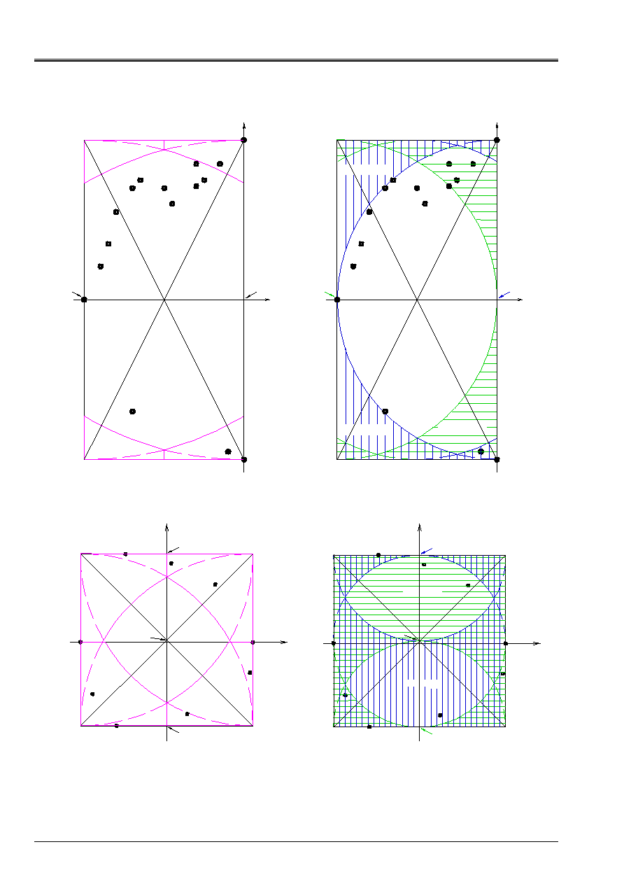
General presentation of the calculation of the circumscribed circle
The method that we use is an exact method which breaks up into four stages.
Stage 1
We frame the points and we determine the co-ordinates of the four corners of the framework in
identify
)
,
,
0
(
v
U
, and co-ordinates of the center of the framework
O
cf [Figure 5.1-a] and [Figure 5.1-c]. In
particular case where the framework summarizes with a horizontal line or vertical it half length of the line
is equal to the half amplitude of shearing.
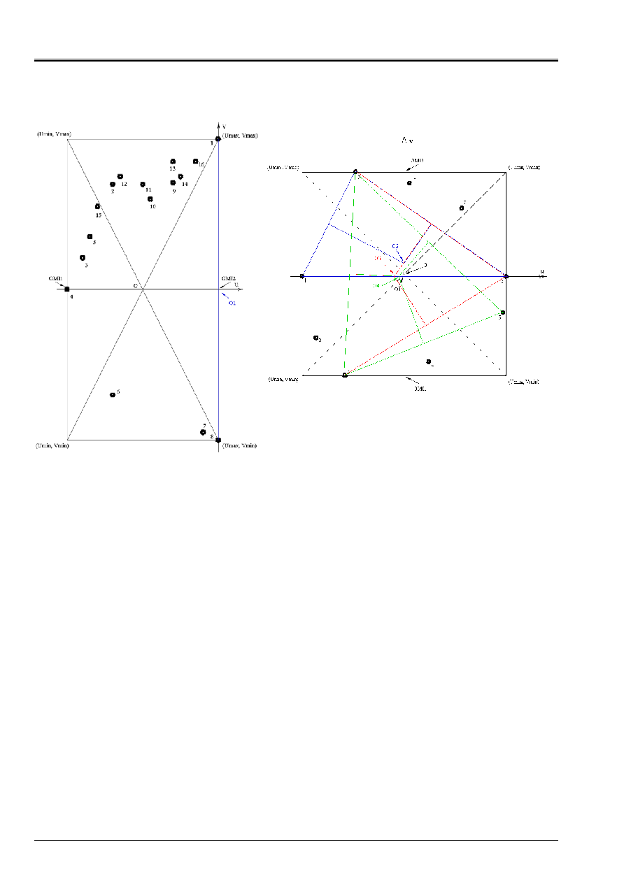
Stage 2
The objective of the second stage is to select the two most distant points. In order to not
to examine the distance between all the possible pairs of points, we build four sectors,
cf [Figure 5.1-a] and [Figure 5.1-c]. These sectors are at the four corners of the framework and are delimited
on the one hand, by the contour of the framework and on the other hand, by an arc of circle whose center is the opposite corner
and the radius the large side of the framework which in fact undervalues the distance between the two most distant points.
Finally, we evaluate the distances between the points of the four sectors two to two:
distances between the points of sector 1 and the points of sector 2;
distances between the points of sector 1 and the points of sector 3;
distances between the points of sector 1 and the points of sector 4;
distances between the points of sector 2 and the points of sector 3;
distances between the points of sector 2 and the points of sector 4;
distances between the points of sector 3 and the points of sector 4.
In the particular case where the report/ratio on the small side of the framework on the large side is strictly lower than
4
3
we do not evaluate the distances between the points belonging to sectors 1 and 2 nor them
distances between the points of sectors 3 and 4, case of the example of [Figure 5.1-a].
Stage 3
In the third stage we build the fields 1 and 2 in which we will seek them
points which are apart from the initial circumscribed circle, cf Etape 4. The constitution of fields 1
and 2 be to reduce the number of points to be explored at the time of stage 4. Principles of
constructions of these two fields are as follows.
1) From the points mediums on the two large sides of the framework (
1
Omi
and
2
Omi
, cf [Figure 5.1-b]
and [Figure 5.1-d]) we trace an arc of circle whose radius corresponds to undervaluing
value of the half amplitude of shearing and is equal to the half length on the large side of
tally.
2) Center of the framework
O
we trace four arcs of circle whose radius is also it
undervaluing value of the half amplitude of shearing.
If
I
O
the center of the circle circumscribes initial A a component according to the axis
U
who places it between
1
Omi
and
O
, then if there is a point of which the distance to
I
O
is higher than
I
R
the radius of the circumscribed circle
initial, it can be only in field 1, cf [Figure 5.1-b].
Code_Aster
®
Version
7.4
Titrate:
Multiaxial criteria of priming in fatigue to great number of cycle
Date
:
01/09/05
Author (S):
J. ANGLES
Key
:
R7.04.04-A
Page
:
16/36
Manual of Reference
R7.04 booklet: Evaluation of the damage
HT-66/05/002/A
2
3
4
5
6
9
10
12
13
14
15
11
U
v
Sector 2
1
16
Sector 1
O
OMI1
OMI2
Sector 4
Sector 3
7
8
(Umin, Vmax)
(Umax, Vmax)
(Umin, Vmin)
(Umax, Vmin)
Appear 5.1-a: Exemple1, localization
sectors
2
3
4
5
6
9
10
12
13
14
15
11
U
1
16
O
OMI1
OMI2
8
(Umin, Vmax)
(Umin, Vmin)
(Umax, Vmin)
7
v
(Umax, Vmax)
FIELD 2
FIELD 2
FIELD 1
FIELD 1
Appear 5.1-b: Exemple1, localization
fields
(Umin, Vmax)
OMI1
OMI2
v
U
Sector 1
1
2
3
4
Sector 4
5
6
Sector 3
7
8
Sector 2
9
O
(Umin, Vmin)
(Umax, Vmin)
(Umax, Vmax)
Appear 5.1-c: Exemple2, localization
sectors
(Umin, Vmax)
OMI1
OMI2
v
U
1
2
3
4
5
6
7
8
9
(Umin, Vmin)
(Umax, Vmax)
(Umax, Vmin)
O
FIELD 1
FIELD 2
Appear 5.1-d: Exemple2, localization
fields

Code_Aster
®
Version
7.4
Titrate:
Multiaxial criteria of priming in fatigue to great number of cycle
Date
:
01/09/05
Author (S):
J. ANGLES
Key
:
R7.04.04-A
Page
:
17/36
Manual of Reference
R7.04 booklet: Evaluation of the damage
HT-66/05/002/A
Stage 4
The goal of the fourth stage is to find the circle circumscribed by the method of the circle passing by
three points, cf [§5.2]. With this intention, we calculate the point medium
1
O
associated the two points more
moved away that we note
1
P
and
2
P
, we deduce the value from it from a first noted radius
1
R
. In
function of the position of
1
O
compared to the large axis of the framework passing in its center, us
let us seek either in field 1, or in field 2, if there is a point located at a distance
higher than the half outdistances measured between the two most distant points
1
P
and
2
P
. Let us note
3
P
such a point. If there is no point such as
3
P
then it half amplitude of shearing is equal to
1
R
,
cf [Figure 5.1-c]. On the other hand, if
3
P
exist we seek the co-ordinates of the point located at equal
outdistance
1
P
,
2
P
and
3
P
; we note this point
2
O
. We obtain a new radius thus,
2
R
thus new a half amplitude of shearing. Again, according to the position of
2
O
by
report/ratio with the large axis of the framework passing in its center, we seek either in field 1, or
in field 2, if there is a point located at a distance higher than
2
R
of
2
O
. Let us note
4
P
such
not. If there is no point such as
4
P
then it half amplitude of shearing is equal to
2
R
. In
revenge, if
4
P
exist we seek the smallest circle circumscribed at the four points:
1
P
,
2
P
,
3
P
and
4
P
by using the method of the circle successively passing by three points, cf [§5.2]. That us
provides a new center
3
O
and a new radius
3
R
. As previously, according to
position of
3
O
compared to the large axis of the framework passing in its center, we seek is in
field 1, is in field 2, if there is a point located at a distance higher than
3
R
of
3
O
.
Let us note
5
P
such a point. If there is no point such as
5
P
then it half amplitude of shearing is
equalize with
3
R
. On the other hand if a point such as
5
P
exist we have five points, if we want to use
the preceding method, where there are only four points concerned, it is necessary to eliminate one from the five
points. That cannot be the last:
5
P
, therefore we preserve preceding iteration the three
points which made it possible to determine
3
O
and
3
R
, i.e. the smallest circumscribed circle. Let us suppose
that
1
P
that is to say thus eliminated. We thus seek the smallest circle circumscribed at the four points:
2
P
,
3
P
,
4
P
and
5
P
by using the method of the circle successively passing by three points, cf [§5.2].
That provides us a new center
4
O
and a new radius
4
R
. According to the position of
4
O
compared to the large axis of the framework passing in its center, we seek either in field 1, or
in field 2, if there is a point located at a distance higher than
4
R
of
4
O
. If it is not the case
the half amplitude of shearing is equal to
4
R
and the circle circumscribes has as a center
4
O
,
cf [Figure 5.1-f]. Contrary, if such a point exists we remake an iteration identical to
the preceding one.
Code_Aster
®
Version
7.4
Titrate:
Multiaxial criteria of priming in fatigue to great number of cycle
Date
:
01/09/05
Author (S):
J. ANGLES
Key
:
R7.04.04-A
Page
:
18/36
Manual of Reference
R7.04 booklet: Evaluation of the damage
HT-66/05/002/A
Appear 5.1-e: Exemple1, search of the circle
circumscribed
Appear 5.1-f: Exemple2, search of the circumscribed circle
Code_Aster
®
Version
7.4
Titrate:
Multiaxial criteria of priming in fatigue to great number of cycle
Date
:
01/09/05
Author (S):
J. ANGLES
Key
:
R7.04.04-A
Page
:
19/36
Manual of Reference
R7.04 booklet: Evaluation of the damage
HT-66/05/002/A
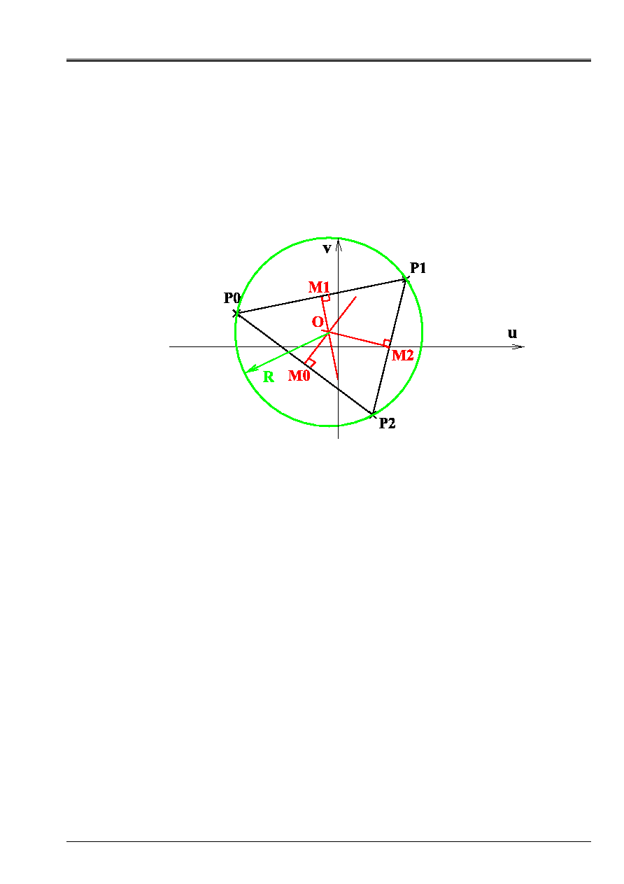
5.2
Description of the method of the circle passing by three points
In this paragraph we will treat the general case, then the particular cases.
5.2.1 Case
General
To determine the circumscribed circle at three points
0
P
,
1
P
and
2
P
, cf [Figure 5.2.1-a], we proceed
in three stages.
Appear 5.2.1-a: Determination of the circle passing by three points
Stage 1
We calculate the co-ordinates of the three points mediums:
0
M
,
1
M
and
2
M
, cf [Figure 5.2.1-a].
Stage 2
We determine the normals passing by the three points mediums
:
0
M
,
1
M
and
2
M
,
cf [Figure 5.2.1-a]. These normals are of the straight lines of the type
B
U
has
v
+
=
where
has
and
B
are constants
that it is possible to calculate with the co-ordinates of the points
0
P
,
1
P
,
2
P
,
0
M
,
1
M
and
2
M
.
Let us describe, now, the manner of determining these normals.
1) Normal with the segment
0
P
1
P
passing by
1
M
We determine the punctual coordinates
'1
M
by rotation of 90° of the segment
0
P
1
M
:
(
)
(
)
1
0
1
1
0
1
1
1
M
P
M
M
P
M
M
M
U
U
V
V
V
V
U
U
-
+
=
-
+
=
éq
5.2.1-1
where
K
U
and
K
V
with
0
,
1
,
1
P
M
M
K
=
the components represent
U
and
v
points
'
1
M
,
1
M
and
0
P
. We deduce the constants from them
0
has
and
0
B
line representing the normal with the segment
0
P
1
P
passing by
1
M
:

Code_Aster
®
Version
7.4
Titrate:
Multiaxial criteria of priming in fatigue to great number of cycle
Date
:
01/09/05
Author (S):
J. ANGLES
Key
:
R7.04.04-A
Page
:
20/36
Manual of Reference
R7.04 booklet: Evaluation of the damage
HT-66/05/002/A
(
) (
)
(
) (
)
1
1
1
1
1
1
0
1
1
1
1
0
M
M
M
M
M
M
M
M
M
M
U
U
V
U
V
U
B
U
U
V
V
has
-
-
=
-
-
=
éq
5.2.1-2
In the particular case where
(
)
0
1
1
=
-
M
M
U
U
, we force
0
has
and
0
B
with zero and we obtain them
co-ordinates of the center
O
circle circumscribed at the points
0
P
,
1
P
and
2
P
by a specific method
described in the paragraph [§5.2.2].
2) Normal with the segment
0
P
2
P
passing by
0
M
We determine the punctual coordinates
'0
M
by rotation of 90° of the segment
0
P
0
M
:
(
)
(
)
0
0
0
0
0
0
0
0
M
P
M
M
P
M
M
M
U
U
V
V
V
V
U
U
-
+
=
-
+
=
éq
5.2.1-3
where
K
U
and
K
V
with
0
,
0
,
0
P
M
M
K
=
the components represent
U
and
v
points
'0
M
,
0
M
and
0
P
. We deduce the constants from them
1
has
and
1
B
line representing the normal with the segment
0
P
2
P
passing by
0
M
:
(
) (
)
(
) (
)
0
0
0
0
0
0
1
0
0
0
0
1
M
M
M
M
M
M
M
M
M
M
U
U
V
U
V
U
B
U
U
V
V
has
-
-
=
-
-
=
éq
5.2.1-4
In the particular case where
(
)
0
0
0
=
-
M
M
U
U
, we force
1
has
and
1
B
with zero and we obtain them
co-ordinates of the center
O
circle circumscribed at the points
0
P
,
1
P
and
2
P
by a specific method
described in the paragraph [§5.2.2].
3) Normal with the segment
1
P
2
P
passing by
2
M
We determine the punctual coordinates
'2
M
by rotation of 90° of the segment
1
P
2
M
:
(
)
(
)
2
1
2
2
1
2
2
2
M
P
M
M
P
M
M
M
U
U
V
V
V
V
U
U
-
+
=
-
+
=
éq
5.2.1-5
where
K
U
and
K
V
with
1
,
2
,
2
P
M
M
K
=
the components represent
U
and
v
points
'2
M
,
2
M
and
1
P
. We deduce the constants from them
2
has
and
2
B
line representing the normal with the segment
1
P
2
P
passing by
2
M
:
(
) (
)
(
) (
)
2
2
2
2
2
2
2
2
2
2
2
2
M
M
M
M
M
M
M
M
M
M
U
U
V
U
V
U
B
U
U
V
V
has
-
-
=
-
-
=
éq
5.2.1-6
In the particular case where
(
)
0
2
2
=
-
M
M
U
U
, we force
2
has
and
2
B
with zero and we obtain them
co-ordinates of the center
O
circle circumscribed at the points
0
P
,
1
P
and
2
P
by a specific method
described in the paragraph [§5.2.2].
Code_Aster
®
Version
7.4
Titrate:
Multiaxial criteria of priming in fatigue to great number of cycle
Date
:
01/09/05
Author (S):
J. ANGLES
Key
:
R7.04.04-A
Page
:
21/36
Manual of Reference
R7.04 booklet: Evaluation of the damage
HT-66/05/002/A
Stage 3
In the general case, we deduce from the constants
0
has
,
0
B
,
1
has
,
1
B
,
2
has
and
2
B
co-ordinates of
center
O
circle circumscribed at the points
0
P
,
1
P
and
2
P
from three manner different. Let us note
0
O
,
1
O
and
2
O
the same center
O
, obtained in three different ways, and
K
U
and
K
V
, where
2
1
0
,
,
O
O
O
K
=
,
the components represent
U
and
v
points
0
O
,
1
O
and
2
O
:
(
) (
)
(
) (
)
1
0
0
1
1
0
1
0
0
1
0
0
has
has
B
has
B
has
V
has
has
B
B
U
O
O
-
-
=
-
-
=
éq
5.2.1-7
(
) (
)
(
) (
)
2
0
0
2
2
0
2
0
0
2
1
1
has
has
B
has
B
has
V
has
has
B
B
U
O
O
-
-
=
-
-
=
éq
5.2.1-8
(
) (
)
(
) (
)
2
1
1
2
2
1
2
1
1
2
2
2
has
has
B
has
B
has
V
has
has
B
B
U
O
O
-
-
=
-
-
=
éq
5.2.1-9
After having checked that equalities:
2
1
0
O
O
O
U
U
U
and
2
1
0
O
O
O
V
V
V
are satisfied us
let us determine the radius of the circle circumscribed by calculating the distance enters
O
and one of the three points
0
P
,
1
P
or
2
P
.
5.2.2 Case
private individuals
In this paragraph we treat the three particular cases of stage 2 of the paragraph [§5.2.1].
Particular case where
(
)
0
1
1
=
-
M
M
U
U
In this case we obtain the components immediately
U
and
v
center
O
by:
(
) (
)
2
1
1
2
2
1
1
has
has
B
has
B
has
V
U
U
O
M
O
-
-
=
=
éq
5.2.2-1
Particular case where
(
)
0
0
0
=
-
M
M
U
U
Here components
U
and
v
center
O
are given by:
(
) (
)
2
0
0
2
2
0
0
0
has
has
B
has
B
has
V
U
U
O
M
-
-
=
=
éq
5.2.2-2
Particular case where
(
)
0
2
2
=
-
M
M
U
U
In this last case, them
U
and
v
center
O
are given by:
(
) (
)
1
0
0
1
1
0
2
0
has
has
B
has
B
has
V
U
U
O
M
-
-
=
=
éq
5.2.2-3
The value of the radius of the circumscribed circle is obtained same manner as in the general case;
i.e., while calculating the distance enters
O
and one of the three points
0
P
,
1
P
or
2
P
.

Code_Aster
®
Version
7.4
Titrate:
Multiaxial criteria of priming in fatigue to great number of cycle
Date
:
01/09/05
Author (S):
J. ANGLES
Key
:
R7.04.04-A
Page
:
22/36
Manual of Reference
R7.04 booklet: Evaluation of the damage
HT-66/05/002/A
5.3
Criteria with critical plans
In this paragraph we give the list of the criteria with critical plans, cf [bib3], which are
programmed as well as a brief description.
Notation:
*
N
: normal in the plan in which the amplitude of shearing is maximum;
)
(
N
: amplitude of shearing in a plan of normal
NR
;
)
(
max
N
NR
: maximum normal stress within normal
NR
during the cycle;
0
: limit of endurance in alternate pure shearing;
0
D
: limit of endurance in alternate pure traction and compression;
)
(
N
m
NR
: average normal stress within normal
NR
during the cycle;
)
(
max
N
: maximum normal deformation within normal
NR
during the cycle;
)
(
N
m
: average normal deformation within normal
NR
during the cycle;
P
: hydrostatic pressure;
p
C
: harmful effect of pre-work hardening in controlled deformation,
1
p
C
.
Criterion of MATAKE
B
NR
has
+
*)
(
2
*)
(
max
N
N
éq 5.3-1
where
has
and
B
are two constant data by the user, they depend on the characteristics
materials and are worth:
.
2
2
0
0
0
0
=
-
=
B
D
D
has
Moreover, we define an equivalent stress within the meaning of MATAKE, noted
*)
(
N
eq
:
,
*)
(
2
*)
(
*)
(
max
T
F
NR
has
C
p
eq
+
=
N
N
N
where
T
F
represent the report/ratio of the limits of endurance in alternate bending and torsion.
Criterion of DANG VAN
B
P
has
+
2
*)
(N
éq 5.3-2
where
has
and
B
are two constant data by the user, they depend on the characteristics
materials and are worth:
(
)
(
)
(
)
.
2
2
2
2
3
1
1
2
2
1
1
2
×
+
-
=
-
-
-
×
=
m
m
m
B
has
Moreover, we define an equivalent stress within the meaning of DANG VAN, noted
*)
(N
eq
:
T
C
P
has
C
p
eq
+
=
2
*)
(
*)
(
N
N
,
where
T
C
represent the report/ratio of the limits of endurance in alternate shearing and traction.

Code_Aster
®
Version
7.4
Titrate:
Multiaxial criteria of priming in fatigue to great number of cycle
Date
:
01/09/05
Author (S):
J. ANGLES
Key
:
R7.04.04-A
Page
:
23/36
Manual of Reference
R7.04 booklet: Evaluation of the damage
HT-66/05/002/A
5.4
A number of cycles to the rupture and damage
From
*)
(N
eq
and from a curve of Wöhler we deduct the number of cycles to the rupture:
*)
(N
NR
, then the damage corresponding to a cycle:
*)
(
1
*)
(
N
N
NR
D
=
.
5.5
Size and components introduced into Code_Aster
The computed values are stored at the points of Gauss or the nodes according to the option selected. One
sizes and of the components were introduced into the catalog of the sizes (file:
grandeur_simple__.cata). Components of the size
FACY_R
(Cyclic Fatigue) are described
in [Table 5.5-1].
DTAUM1
first value of the half amplitude max of shearing in the critical plan
VNM1X
component X of the normal vector in the plan criticizes dependant A
DTAUM1
VNM1Y
component of the normal vector in the plan criticizes dependant A there
DTAUM1
VNM1Z
component Z of the normal vector in the plan criticizes dependant A
DTAUM1
SINMAX1
normal maximum stress in the plan criticizes agent with
DTAUM1
SINMOY1
normal mean stress in the plan criticizes agent with
DTAUM1
EPNMAX1
normal maximum deformation in the plan criticizes agent with
DTAUM1
EPNMOY1
average maximum deformation in the plan criticizes agent with
DTAUM1
SIGEQ1
Stress equivalent within the meaning of the criterion selected agent to
DTAUM1
NBRUP1
a number of cycles before rupture (function of
SIGEQ1
and of a curve of Wöhler)
ENDO1
damage associated with
NBRUP1
(ENDO1=1/NBRUP1)
DTAUM2
second value of the half amplitude max of shearing in the critical plan
VNM2X
component X of the normal vector in the plan criticizes dependant A
DTAUM2
VNM2Y
component of the normal vector in the plan criticizes dependant A there
DTAUM2
VNM2Z
component Z of the normal vector in the plan criticizes dependant A
DTAUM2
SINMAX2
normal maximum stress in the plan criticizes agent with
DTAUM2
SINMOY2
normal mean stress in the plan criticizes agent with
DTAUM2
EPNMAX2
normal maximum deformation in the plan criticizes agent with
DTAUM2
EPNMOY2
average maximum deformation in the plan criticizes agent with
DTAUM2
SIGEQ2
Stress equivalent within the meaning of the criterion selected agent to
DTAUM2
NBRUP2
a number of cycles before rupture (function of
SIGEQ2
and of a curve of Wöhler)
ENDO2
damage associates
NBRUP2
(ENDO2=1/NBRUP2)
Table 5.5-1: Components specific to multiaxial cyclic fatigue

Code_Aster
®
Version
7.4
Titrate:
Multiaxial criteria of priming in fatigue to great number of cycle
Date
:
01/09/05
Author (S):
J. ANGLES
Key
:
R7.04.04-A
Page
:
24/36
Manual of Reference
R7.04 booklet: Evaluation of the damage
HT-66/05/002/A
6
Criteria with variable amplitude
The criteria with variable amplitude are implemented when the loading is not periodic. When
the loading is not periodic it is necessary to break up the way of loading undergone by
structure in elementary under-cycles using a method of counting of cycles. If it
loading is nonradial it does not have there tested multiaxial method of counting. Consequently
we choose, as in the literature, to use the method of counting RAINFLOW [bib7] which has
requirement in input for a scalar. This is why we reduce to a dimension the cission, which is
orthogonal projection of the vector forced on a plan, by projecting the point of the vector cission on one
or two axes. Another important difference with the criteria in critical plan is that it is not
the amplitude of shearing which makes it possible to select the critical plan but the office plurality of damage which
result from the elementary under-cycles.
The method of projection that we use is clarified in chapters 7 and 8. In the continuation us
let us describe the way in which we made evolve/move the criteria of MATAKE and DANG VAN for
to adapt to the cases where the loading is not periodical.
6.1
Criterion of modified MATAKE
In the context of the office plurality of damage and a periodic loading, the criterion of MATAKE [bib6],
is written in the following way:
()
()
*
max
*
2
N
NR
has
N
C
p
eq
R
R
+
=
éq
6.1-1
where
eq
represent the stress equivalent within the meaning of the criterion of MATAKE and with:
*
NR
normal in the plan for which the amplitude of shearing is maximum;
()
2
*
NR
maximum half-amplitude of shearing;
has
constant which perhaps defined by a pure shear test alternated and in
alternate traction and compression or by a test in alternate traction and compression and in
nonalternate traction and compression;
()
*
max
N
NR
R
maximum normal stress within normal
*
NR
during the cycle;
p
C
harmful effect of pre-work hardening in controlled deformation
1
p
C
.
To calculate the cumulated damage if the loading is not periodical the first stage
consist in determining the cission (vector shearing) in a plan of normal
NR
at every moment
loading. The technique which is used with this intention is described in the reference [bib6]. In
second stage we start by reducing the history of the cission to a function
unidimensional of time by projecting the point of the vector cission on one or two axes defined in
the plan of normal
NR
considered, cf chapter 7 and 8. Thus the evolution of the projected cission is summarized with
the relation:
)
(T
F
p
=
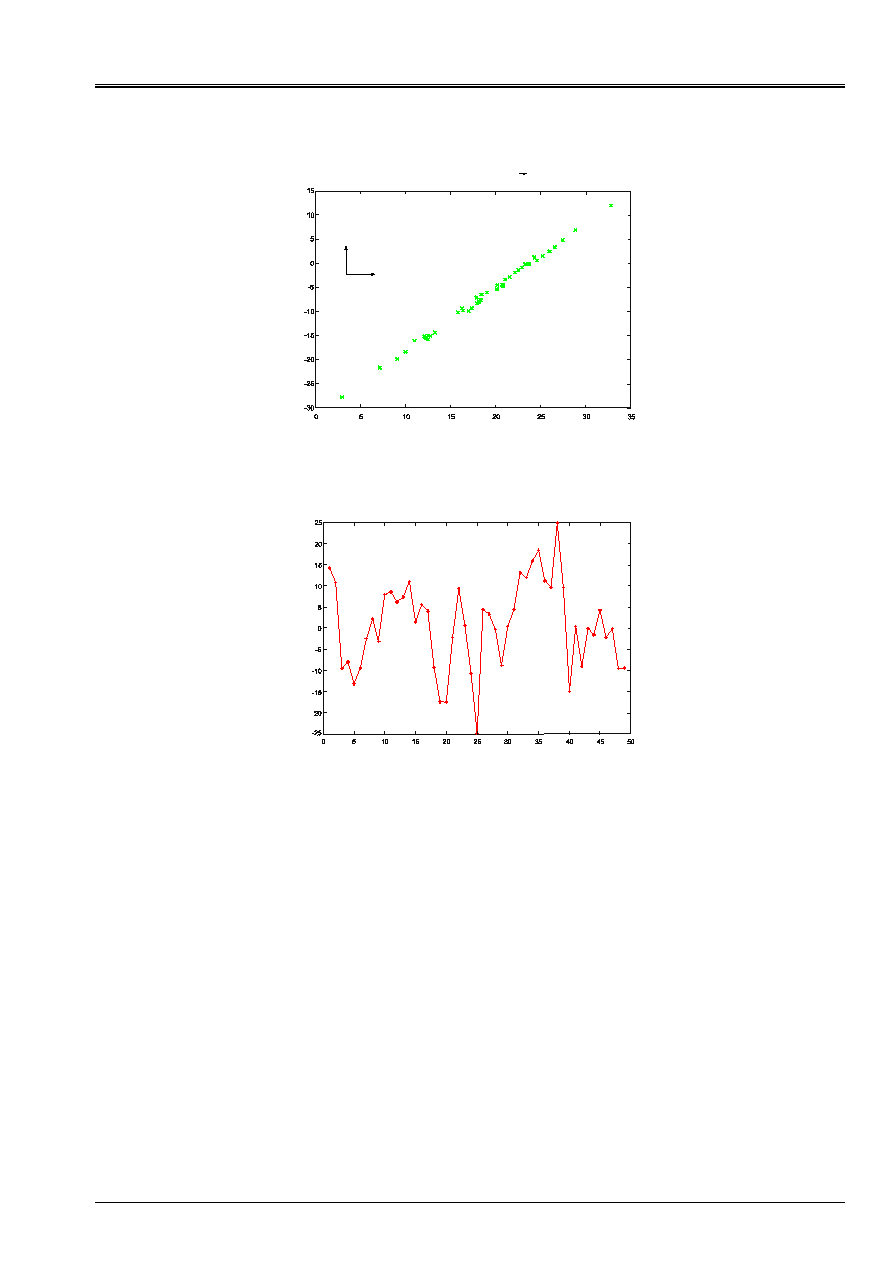
what makes it possible to use the method of counting RAINFLOW. On the figure
[Figure 6.1-a] we show the values reached by the end of the vector shearing in a plan
of normal
NR
before projection on an axis or two axes and the figure [Figure 6.1-b] these same
values after projection on an axis. This stage it is necessary for us to introduce the concept of stress
equivalent elementary
ieq
. Practically this concept with the same significance as the concept of
equivalent stress defined by the relation [éq 6.1-1], but it applies to the under-cycles
elementary resulting from the method of counting RAINFLOW. Thus starting from the projected cission
p
we calculate elementary equivalent stresses
ieq
.
Code_Aster
®
Version
7.4
Titrate:
Multiaxial criteria of priming in fatigue to great number of cycle
Date
:
01/09/05
Author (S):
J. ANGLES
Key
:
R7.04.04-A
Page
:
25/36
Manual of Reference
R7.04 booklet: Evaluation of the damage
HT-66/05/002/A
v
U
Cission in a plan of normal N (MPa)
Appear 6.1-a: Points of the vector cission before projection
Sequence number
p
Cission projected on axis 1 (MPa)
Appear 6.1-b: Points of the vector cission after projection on an axis
Method RAINFLOW breaks up
)
(T
F
p
=
in periodic elementary under-cycles and breaks
the history of the loading, as we show it on the figure [Figure 6.1-c]. Thus, for one
normal
NR
data method RAINFLOW provides for each elementary under-cycle two values,
points high and low, of the point of the vector cission
()
N
I
p
R
1
and
()
N
I
p
R
2
associated two values of
maximum normal stress
()
N
NR
I
R
1
max
and
()
N
NR
I
R
2
max
.

Code_Aster
®
Version
7.4
Titrate:
Multiaxial criteria of priming in fatigue to great number of cycle
Date
:
01/09/05
Author (S):
J. ANGLES
Key
:
R7.04.04-A
Page
:
26/36
Manual of Reference
R7.04 booklet: Evaluation of the damage
HT-66/05/002/A
Under elementary cycles (MPa)
Numbers of the points
p
38
40
41
42
43
44
45
46
47
48
1
3
4
5
9
8
11
12
14
15
16
20
25
22
26
29
32
33
35
37
Sequence numbers or
numbers of the moments
1
2
3
4
5
6
7
8
9
10
11
12
13
14
15
Numbers of under cycles
Appear 6.1-c: Fifteen elementary under-cycles after processing by method RAINFLOW
For the criterion of MATAKE we define the elementary equivalent stress in the manner
following:
(
) (
)
(
)
0
,
)
(
,
)
(
2
)
(
,
)
(
)
(
,
)
(
)
(
2
1
2
1
2
1
max
max
N
NR
N
NR
Max
has
N
N
Min
N
N
Max
C
N
I
I
I
p
I
p
I
p
I
p
p
ieq
R
R
R
R
R
R
R
+
-
=
éq 6.1-2
For the office plurality of damage, this elementary equivalent stress is to be used with a curve of
tire in shearing. If one uses a curve of fatigue in traction compression it is necessary to multiply
[éq 6.1-2] by a corrective coefficient which corresponds to the report/ratio of the limits of endurance in bending and in
alternate torsion and which we note
:
(
) (
)
(
)
+
-
=
0
,
)
(
,
)
(
2
)
(
,
)
(
)
(
,
)
(
)
(
2
1
2
1
2
1
max
max
N
NR
N
NR
Max
has
N
N
Min
N
N
Max
C
N
I
I
IP
IP
IP
IP
p
ieq
R
R
R
R
R
R
R
éq 6.1-3

Code_Aster
®
Version
7.4
Titrate:
Multiaxial criteria of priming in fatigue to great number of cycle
Date
:
01/09/05
Author (S):
J. ANGLES
Key
:
R7.04.04-A
Page
:
27/36
Manual of Reference
R7.04 booklet: Evaluation of the damage
HT-66/05/002/A
From
)
(N
ieq
R
and from a curve of Wöhler we deduct the number of cycles to the rupture
)
(N
NR
I
R
and elementary damage
)
(
1
)
(
N
NR
N
D
I
I
R
R
=
agent with an elementary under-cycle.
We use a linear office plurality of damage. That is to say
K
the number of elementary under-cycles, for
a normal
NR
fixed, the cumulated damage is equal to:
=
=
K
I
I
N
D
N
D
1
)
(
)
(
R
R
éq
6.1-4
To determine the normal vector
*
NR
corresponding to the maximum cumulated damage it is enough to make
to vary
NR
and to calculate [éq 6.1-4]. The normal vector
*
NR
corresponding to the maximum cumulated damage
is then given by:
(
)
)
(
)
(
*
N
D
Max
N
D
N
R
R
R
=
6.2
Criterion of modified DANG VAN
Within the framework of the damage and a periodic loading, the criterion of DANG VAN is written:
P
has
N
C
N
p
eq
+
=
2
)
(
)
(
*
*
R
R
where
eq
represent the stress equivalent within the meaning of the criterion of DANG VAN and with:
*
NR
normal in the plan for which the amplitude of shearing is maximum;
()
2
*
NR
maximum half-amplitude of shearing;
has
constant which perhaps defined by a pure shear test alternated and in
alternate traction and compression or by a test in alternate traction and compression and in
nonalternate traction and compression;
P
maximum hydrostatic pressure during the cycle;
p
C
harmful effect of pre-work hardening in controlled deformation
1
p
C
.
When the loading is not periodical, we calculate the damage by the same process
that that used for the criterion of MATAKE. The only difference lies in the definition of
elementary equivalent stress:
(
) (
)
(
)
0
,
)
(
,
)
(
2
)
(
,
)
(
)
(
,
)
(
)
(
2
1
2
1
2
1
N
P
N
P
Max
has
N
N
Min
N
N
Max
C
N
I
I
I
p
I
p
I
p
I
p
p
ieq
R
R
R
R
R
R
R
+
-
=
éq
6.2-1
where
I
P
1
and
I
P
2
the two values of the hydrostatic pressure represent attached to each
elementary under-cycle. This elementary equivalent stress is to be used with a curve of
tire in shearing. If one must employ a curve of fatigue in traction compression it is
necessary to multiply [éq 6.2-1] by the corrective coefficient
:
(
) (
)
(
)
+
-
=
0
,
)
(
,
)
(
2
)
(
,
)
(
)
(
,
)
(
)
(
2
1
2
1
2
1
N
P
N
P
Max
has
N
N
Min
N
N
Max
C
N
I
I
IP
IP
IP
IP
p
ieq
R
R
R
R
R
R
R
After having defined the criteria of MATAKE and DANG VAN within the framework of the office plurality of damage and
of a nonperiodic loading, it remains us to specify the technique of projection that us
let us propose.
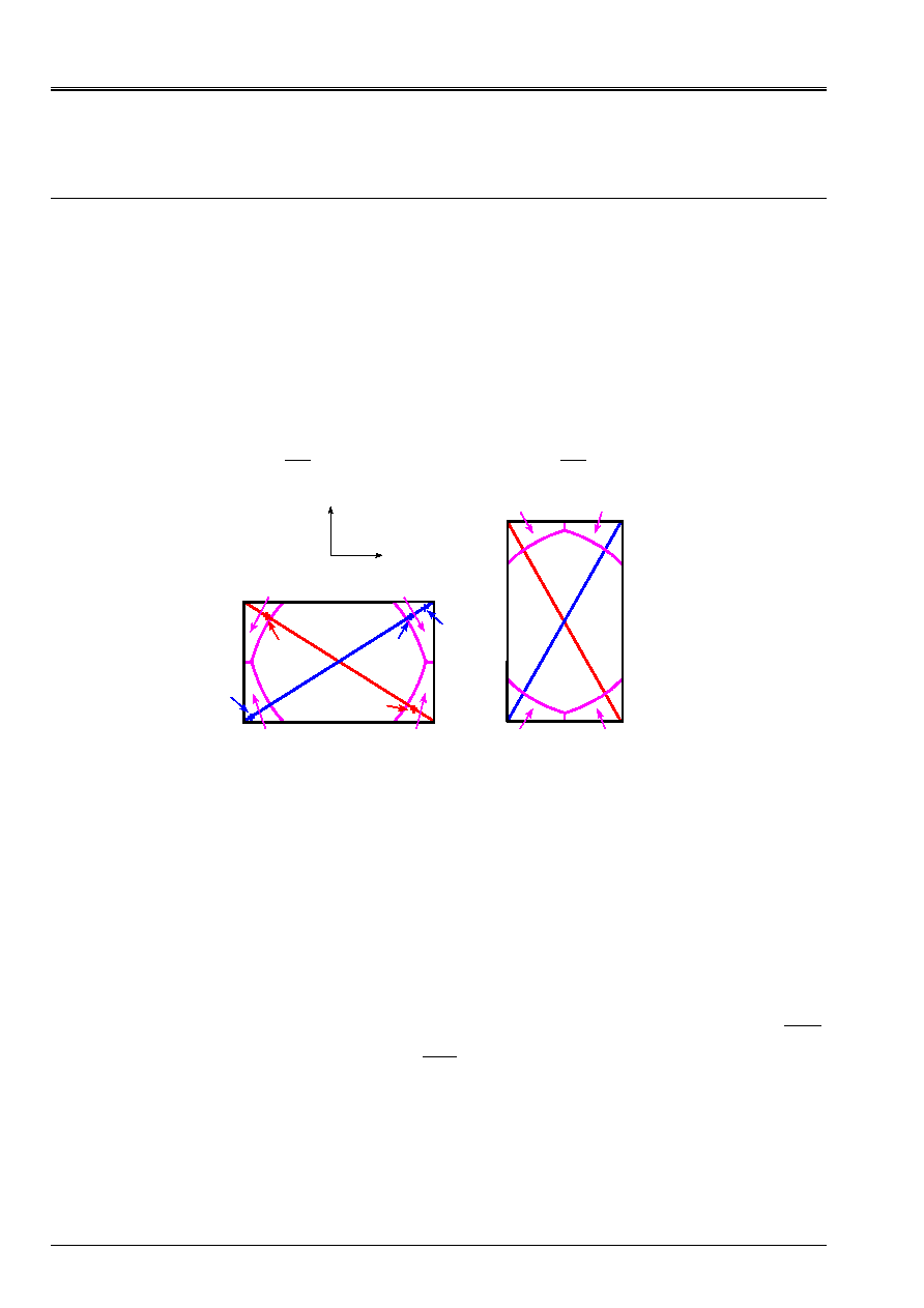
Code_Aster
®
Version
7.4
Titrate:
Multiaxial criteria of priming in fatigue to great number of cycle
Date
:
01/09/05
Author (S):
J. ANGLES
Key
:
R7.04.04-A
Page
:
28/36
Manual of Reference
R7.04 booklet: Evaluation of the damage
HT-66/05/002/A
7
Choice of the axes of projection
With regard to the projection of the end of the vector cission we propose two options:
1) a projection on an axis,
2) a projection on two axes.
The axis of option 1 is in the same way given that the first axis of option 2. The second axis of
option 2 is orthogonal with the first axis of this option.
7.1
Projection on an axis
We place ourselves in a plan of normal
NR
data where each point represents the position of
point vector shearing at one moment, for more details to see the reference [bib6]. In this plan
we build the smallest framework which contains all the points representing the end of the vector
cission at every moment. The two diagonals of the framework enable us to define two axes: axis 1
corresponds to the segment
AC
, and centers it 2 corresponds to the segment
DB
, cf [Figure 7.1].
axe1
axe2
O
With
B
D
C
Sector Sector
Sector Sector
Appear 7.1-a
Appear 7.1-b
WITH B
D C
axe1
axe2
O
Sector Sector
Sector
Sector
P1
P2
P4
P3
P5
v
U
Figure 7.1: Definition of the axes of projection
We choose a priori the axis of projection among axes 1 and 2 because the diagonal of the framework is
larger than the large side of the framework what has as a virtue to dilate a little the projected points.
In addition the loadings which interest us are of thermal origin with the result that the points
representing the evolution of the point of the vector cission, in the plans of normal
NR
, are more
often aligned on an axis, as we show it on the figure [Figure 6.1-a].
Sectors 1, 2, 3 and 4 are built same manner as in the reference [bib6]. Only them
points which are in these sectors are projected orthogonally on axes 1 and 2.
We define the axis of projection as being the axis on which the distance between two points
projected is largest.
For example, on [Figure 7.1-a] the axis of projection is axis 1 since the length of the segment
4
3
P
P
is greater than the length of the segment
2
1
P
P
. This definition of the axis of projection allows
to make sure that the axis of projection retained will make it possible to account for the amplitude of shearing
projected largest.
According to the presence or absence of points in sectors 1, 2, 3 and 4 determination of
the axis of projection can be immediate, it is then not necessary to implement the procedure
of selection described above. For more details the reader will be able to refer to appendix 1.
A second axis is necessary to distinguish the case where points representing the point of the vector
cission are aligned on an axis of the case where these points describe a circle.
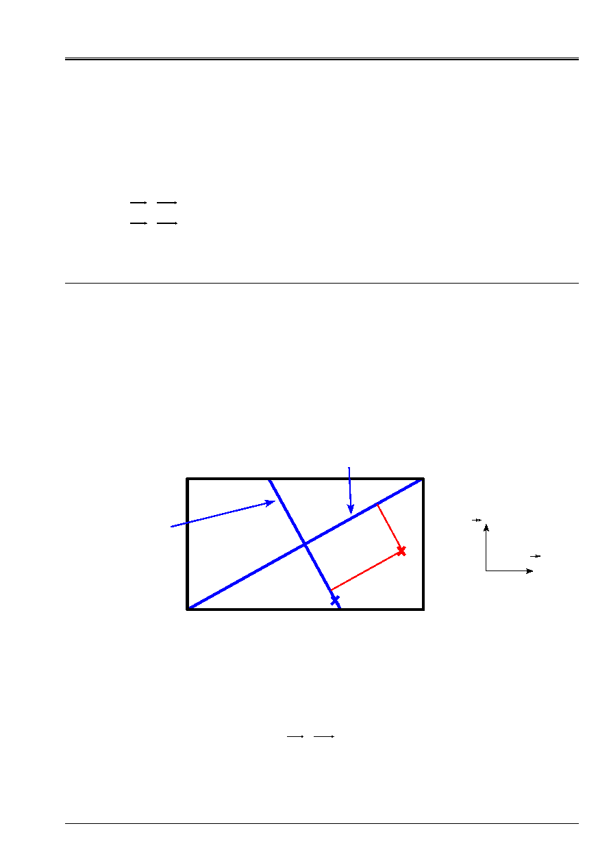
Code_Aster
®
Version
7.4
Titrate:
Multiaxial criteria of priming in fatigue to great number of cycle
Date
:
01/09/05
Author (S):
J. ANGLES
Key
:
R7.04.04-A
Page
:
29/36
Manual of Reference
R7.04 booklet: Evaluation of the damage
HT-66/05/002/A
7.2
Construction of the second axis
The second axis of projection is orthogonal with the initial axis of projection and it passes by the point O.
Since we know the co-ordinates of the points A, B, C and D, to characterize it completely
second axis it is enough to determine the punctual coordinates M such as:
0
.
=
OM
DB
if the initial axis is axis 1,
0
.
=
OM
AC
if the initial axis is axis 2.
8
Projection of shearing
In this chapter we describe the process of projection on the initial axis, or first axis, and the second
center. We remind the meeting that projection on these two axes is orthogonal.
8.1
Case where axis 1 is the initial axis
This case is represented on [Figure 8.1-a]. We in the reference mark place
(
)
N
v
U
O
R
R
R,
,
,
. Definitions
of
ur
,
vr
and
NR
are given in the reference [bib6]. In the plan
()
v
U R
R,
of normal
NR
points A,
B, C, D and O have respectively, for co-ordinates
(
)
max
min
, V
U
,
(
)
max
max
, V
U
,
(
)
min
max
, V
U
,
(
)
min
min
, V
U
and
(
)
O
O
V
U,
.
With
B
D
C
O
M
P
Initial axis
Second axis
P
I
P
S
v
U
Appear 8.1-a: Projection if axis 1 is the initial axis
8.1.1 Determination of the second axis
Here to determine the second axis we solve the equation:
0
.
=
OM
DB
éq
8.1.1-1
where co-ordinates
M
M
V
U,
point M are the unknown factors.
Code_Aster
®
Version
7.4
Titrate:
Multiaxial criteria of priming in fatigue to great number of cycle
Date
:
01/09/05
Author (S):
J. ANGLES
Key
:
R7.04.04-A
Page
:
30/36
Manual of Reference
R7.04 booklet: Evaluation of the damage
HT-66/05/002/A
The equation [éq 8.1.1-1] is also written in the following form:
(
) (
) (
) (
)
0
min
max
min
max
=
-
-
+
-
-
O
M
O
M
V
V
V
V
U
U
U
U
what leads to:
(
)
(
) (
)
O
M
O
M
U
U
V
V
U
U
V
V
-
-
-
-
=
min
max
min
max
By giving a value of
M
U
different from
O
U
we obtain immediately
M
V
.
8.1.2 Projection of an unspecified point on the initial axis
Starting from a point
P
unspecified known, the first stage consists in calculating the co-ordinates of one
not
'
P
such as:
0
.
=
P
P
B
D
While proceeding like previously, we obtain the relation:
(
)
(
) (
)
P
P
P
P
U
U
V
V
U
U
V
V
-
-
-
-
=
min
max
min
max
where
P
V
result from a value from
P
U
different from
P
U
.
In the plan
)
,
(v
U
the initial axis and the segment
P
P
are lines closely connected respectively described by
I
I
B
U
has
v
+
=
and
P
P
B
U
has
v
+
=
, therefore to know the co-ordinates of the point projected on the initial axis
p
P
we solve the equation:
P
P
I
I
B
U
has
B
U
has
+
=
+
where
(
)
(
)
min
max
min
max
U
U
V
V
has
I
-
-
=
,
(
)
(
)
min
max
max
min
min
max
U
U
V
U
V
U
B
I
-
-
=
,
(
)
(
)
P
P
P
P
P
U
U
V
V
has
-
-
=
,
(
)
(
)
P
P
P
P
P
P
P
U
U
V
U
V
U
B
-
-
=
.
One obtains:
p
I
I
p
P
has
has
B
B
U
I
-
-
=
p
I
I
P
P
I
P
has
has
B
has
B
has
V
I
-
-
=
The projection of an unspecified point on the second axis is described in appendix 2.

Code_Aster
®
Version
7.4
Titrate:
Multiaxial criteria of priming in fatigue to great number of cycle
Date
:
01/09/05
Author (S):
J. ANGLES
Key
:
R7.04.04-A
Page
:
31/36
Manual of Reference
R7.04 booklet: Evaluation of the damage
HT-66/05/002/A
8.2
Case where axis 2 is the initial axis
This case is represented on [Figure 8.2-a]. As previously, in the plan
()
v
U R
R,
points A,
B, C, D and O have respectively, for co-ordinates
(
)
max
min
, V
U
,
(
)
max
max
, V
U
,
(
)
min
max
, V
U
,
(
)
min
min
, V
U
and
(
)
O
O
V
U
,
.
With
B
D
C
O
M
P
Initial axis
Second axis
P
I
P
S
v
U
Appear 8.2-a: Projection if axis 2 is the initial axis
8.2.1 Determination of the second axis
Here to determine the second axis we solve the equation:
0
.
=
OM
AC
éq
8.2.1-1
where co-ordinates
)
,
(
M
M
V
U
point M are the unknown factors.
The equation [éq 8.2.1-1] is also written in the following form:
(
) (
) (
) (
)
0
max
min
min
max
=
-
-
+
-
-
O
M
O
M
V
V
V
V
U
U
U
U
what leads to:
(
)
(
) (
)
O
M
O
M
U
U
V
V
U
U
V
V
-
-
-
+
=
min
max
min
max
By giving a value of
M
U
different from
O
U
we obtain immediately
M
V
.
8.2.2 Projection of an unspecified point on the initial axis
Starting from a point
P
unspecified known, the first stage consists in calculating the co-ordinates of one
not
P
such as:
0
.
=
P
P
AC
While proceeding like previously, we obtain the relation:
(
)
(
) (
)
P
P
P
P
U
U
V
V
U
U
V
V
-
-
-
+
=
min
max
min
max
where for a value of
P
U
different from
P
U
we calculate
P
V
.

Code_Aster
®
Version
7.4
Titrate:
Multiaxial criteria of priming in fatigue to great number of cycle
Date
:
01/09/05
Author (S):
J. ANGLES
Key
:
R7.04.04-A
Page
:
32/36
Manual of Reference
R7.04 booklet: Evaluation of the damage
HT-66/05/002/A
In the plan
)
,
(v
U
the initial axis and the segment
P
P
are lines closely connected respectively described by
I
I
B
U
has
v
+
=
and
P
P
B
U
has
v
+
=
, therefore to know the co-ordinates of the point projected on the initial axis
p
P
we solve the equation:
P
P
I
I
B
U
has
B
U
has
+
=
+
where
(
)
(
)
min
max
min
max
U
U
V
V
has
I
-
-
-
=
,
(
)
(
)
min
max
min
min
max
max
U
U
V
U
V
U
B
I
-
-
=
,
(
)
(
)
P
P
P
P
p
U
U
V
V
has
-
-
=
,
(
)
(
)
P
P
P
P
P
P
P
U
U
V
U
V
U
B
-
-
=
.
One obtains:
P
I
I
P
P
has
has
B
B
U
I
-
-
=
,
P
I
I
P
P
I
P
has
has
B
has
B
has
V
I
-
-
=
.
The projection of an unspecified point on the second axis is described in appendix 2.
8.3
Definition of the module and orientation of the axis of projection
We propose to define the sign of the module of the point projected compared to the initial axis. That is to say the reference mark
(
)
N
v
U
O
R
R
R,
,
,
in which the cission evolves/moves. In this reference mark if the component
I
P
U
projected point is
higher or equal to zero the sign of the module is positive, if not it is negative. In short the module and
the sign of the module of the projected point are in the following way defined:
.
0
,
0
2
2
MOD
2
2
MOD
<
+
-
=
+
=
I
I
P
S
I
P
S
I
U
if
COp
COp
P
U
if
COp
COp
P
The definition of the module differentiates the loadings closely connected from the circular loadings. Conformément
with the experiment a circular loading will be regarded as being more damaging that one
loading refines [bib1].
8.4 Components
of
Code_Aster used
VNM1X
component X of the normal vector in the plan of greater damage
VNM1Y
component there of the normal vector in the plan of greater damage
VNM1Z
component Z of the normal vector in the plan of greater damage
ENDO1
The most important damage
9 Conclusion
In this document we presented the criteria of MATAKE and DANG VAN adapted to the office plurality
of damage under periodic and nonperiodic loading.
When the loading is periodic the criteria of MATAKE and DANG VAN are tested by
case tests SSLV135a and SSLV135b. The cases tests SSLV135c and SSLV135d test these two criteria
if the loading is not periodical.
The key words which make it possible to use these two criteria are described in the document [U4.83.02]
devoted to the control
CALC_FATIGUE
. One will be able to also consult the key word factor
CISA_PLAN_CRIT
control
DEFI_MATERIAU
[U4.43.01].

Code_Aster
®
Version
7.4
Titrate:
Multiaxial criteria of priming in fatigue to great number of cycle
Date
:
01/09/05
Author (S):
J. ANGLES
Key
:
R7.04.04-A
Page
:
33/36
Manual of Reference
R7.04 booklet: Evaluation of the damage
HT-66/05/002/A
10 Bibliography
[1]
TAHERI S.: Bibliography on fatigue with great number of cycles, Notes HI-74/94/086/0
[2]
DANG VAN K., GRIVEAU B., MESSAGE O.: There is new multiaxial tires limit criterion:
theory and application. Biaxial and Multiaxial Tires, ED. Brown/Miller, 1989.
[3]
MANDEL J., ZARKA J., HALPHEN B.: Adaptation of an elastoplastic structure to
kinematic work hardening. Mechanical research communications, vol. 4 (5), 1977.
[4]
CLEMENT J.C. : Study and optimization of a method of calculation of fatigue under stresses
multiaxial of variable amplitude, Notes HP-17/97/023/A, June 1997.
[5]
TAHERI S.: The taking into account of a loading with variable amplitude for the calculation of
damage of fatigue in the areas of mixtures Projet FATMAV, Note HT-64/04/011,
December 2004.
[6]
ANGLES J.; Multiaxial criteria of priming in fatigue to great number of cycles, plan
critical, DANG VAN, Project FATMAV, Note HT-64/03/015/A.
[7]
DONORE A.M.; Estimate of the fatigue life to great number of cycles and in
oligocyclic fatigue, Manual of reference of Code_Aster, Document [R7.04.01].
[8]
PAPADOPOULOS INTER-F; Polycyclic fatigue of metals, a new approach, Thesis
presented at the ENPC on December 18, 1987.
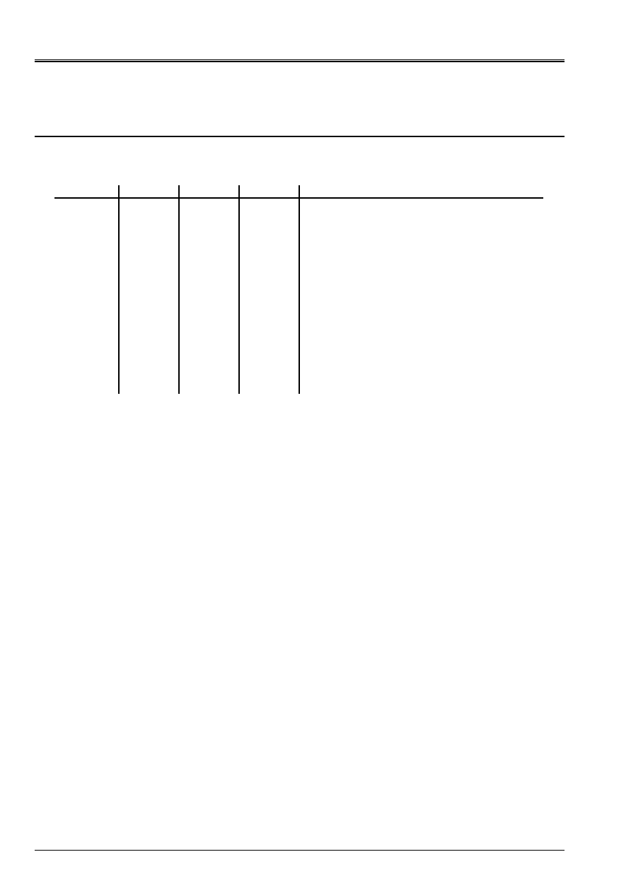
Code_Aster
®
Version
7.4
Titrate:
Multiaxial criteria of priming in fatigue to great number of cycle
Date
:
01/09/05
Author (S):
J. ANGLES
Key
:
R7.04.04-A
Page
:
34/36
Manual of Reference
R7.04 booklet: Evaluation of the damage
HT-66/05/002/A
Appendix 1
The various situations are summarized in [A1-1 Table]. In [A1-1 Table], “0” and “1”
mean respectively that there are no points and that there is at least a point in the indicated sectors.
Sector 1 Sector 3 Sector 2 Sector 4
Center projection
0 0 0 0
Case
impossible.
0 0 0 1
Case
impossible.
0 0 1 0
Case
impossible.
0 0 1 1
Center
1.
0 1 0 0
Case
impossible.
0 1 0 1
Use
of
procedure of selection.
0 1 1 0
Use
of
procedure of selection.
0 1 1 1
Center
1.
1 0 0 0
Case
impossible.
1 0 0 1
Use
of
procedure of selection.
1 0 1 0
Use
of
procedure of selection.
1 0 1 1
Center
1.
1 1 0 0
Center
2.
1 1 0 1
Center
2.
1 1 1 0
Center
2.
1 1 1 1
Use
of
procedure of selection.
A1-1 table: Summary of the situations
The impossible cases result from the way in which the framework and the sectors are built. This construction
makes impossible the presence of points in no or only one sector.

Code_Aster
®
Version
7.4
Titrate:
Multiaxial criteria of priming in fatigue to great number of cycle
Date
:
01/09/05
Author (S):
J. ANGLES
Key
:
R7.04.04-A
Page
:
35/36
Manual of Reference
R7.04 booklet: Evaluation of the damage
HT-66/05/002/A
Appendix 2
The projection of an unspecified point on the second axis is quickly described in this appendix. From one
not
P
unspecified known, we calculate the punctual coordinates
P
such as:
0
.
=
P
P
M
O
After simplification it comes the relation:
(
)
(
) (
)
P
P
O
M
O
M
P
P
U
U
V
V
U
U
V
V
-
-
-
-
=
where a value of
P
U
different from
P
U
us gives
P
V
.
In the plan
)
,
(v
U
the second axis and the segment
P
P
are lines closely connected respectively described by
S
S
B
U
has
v
+
=
and
P
P
B
U
has
v
+
=
, therefore to know the co-ordinates of the point projected on the second axis
p
P
we solve the equation:
P
P
S
S
B
U
has
B
U
has
+
=
+
where
(
)
(
)
O
M
O
M
S
U
U
V
V
has
-
-
=
,
(
)
(
)
O
M
M
O
O
M
S
U
U
V
U
V
U
B
-
-
=
,
(
)
(
)
P
P
P
P
P
U
U
V
V
has
-
-
=
,
(
)
(
)
P
P
P
P
P
P
P
U
U
V
U
V
U
B
-
-
=
.
One obtains:
P
S
S
P
P
has
has
B
B
U
S
-
-
=
,
p
S
S
P
P
S
P
has
has
B
has
B
has
V
S
-
-
=
.

Code_Aster
®
Version
7.4
Titrate:
Multiaxial criteria of priming in fatigue to great number of cycle
Date
:
01/09/05
Author (S):
J. ANGLES
Key
:
R7.04.04-A
Page
:
36/36
Manual of Reference
R7.04 booklet: Evaluation of the damage
HT-66/05/002/A
Intentionally white left page.