
Code_Aster
®
Version
3
Titrate:
Finite elements in accoustics
Date:
31/08/95
Author (S):
F. STIFKENS
Key:
R4.02.01-A
Page:
1/16
Manual of Reference
R4.02 booklet: Accoustics
HP-61/95/070/A
Organization (S):
EDF/EP/AMV
Manual of Reference
R4.02 booklet: Accoustics
Document: R4.02.01
Finite elements in accoustics
Summary:
This document describes in low frequency stationary accoustics the equations used, the formulations
variational which results from this as well as the corresponding translation in finite elements, for each one of
two methods used in Code_Aster: conventional '' formulation " with an unknown factor
p
(acoustic pressure),
and “mixed” formulation with two unknown factors
p, v
(pressure and speed acoustics).

Code_Aster
®
Version
3
Titrate:
Finite elements in accoustics
Date:
31/08/95
Author (S):
F. STIFKENS
Key:
R4.02.01-A
Page:
2/16
Manual of Reference
R4.02 booklet: Accoustics
HP-61/95/070/A
Contents
1 Introduction ............................................................................................................................................ 3
2 Equations and boundary conditions of the problem ................................................................................... 4
2.1 Equations and boundary conditions ................................................................................................. 4
3 conventional Formulation in pressure ........................................................................................................ 6
3.1 Mathematical expression of the problem .......................................................................................... 6
3.2 Discretization by finite elements ...................................................................................................... 6
3.2.1 The matrix of rigidity .............................................................................................................. 7
3.2.2 The matrix of mass .............................................................................................................. 7
3.2.3 The matrix of damping ................................................................................................... 7
3.2.4 The vector source ................................................................................................................... 8
4 mixed Formulation pressure-speed ....................................................................................................... 9
4.1 Mathematical expression of the problem .......................................................................................... 9
4.1.1 Local formulation .................................................................................................................. 9
4.1.2 Mixed variational formulation ............................................................................................. 9
4.2 Discretization by finite elements .................................................................................................... 10
4.2.1 The matrix of rigidity ............................................................................................................ 11
4.2.2 The matrix of mass ............................................................................................................ 12
4.2.3 The matrix of damping ................................................................................................. 12
4.2.4 The vector source ................................................................................................................. 12
5 Controls specific to acoustic modeling ....................................................................... 13
6 Conclusion ........................................................................................................................................... 16
7 Bibliography ........................................................................................................................................ 16

Code_Aster
®
Version
3
Titrate:
Finite elements in accoustics
Date:
31/08/95
Author (S):
F. STIFKENS
Key:
R4.02.01-A
Page:
3/16
Manual of Reference
R4.02 booklet: Accoustics
HP-61/95/070/A
1 Introduction
Options of modeling were developed in Code_Aster, making it possible to study
low frequency stationary acoustic propagation, in closed medium, for fields of
propagation with complex topology, i.e. to solve there under the quoted conditions the equation of
Helmholtz.
The solution by finite elements of this equation can be carried out according to two methods:
·
a first method consists in being fixed like unknown factors of the problem, only them
nodal complex acoustic pressures, is 1 degree of freedom per node [bib1]; it is that
that one qualifies formulation with the finite elements “conventional”,
·
in the second method, called to the finite elements “mixed”, one fixes oneself like unknown factors at
time nodal acoustic pressures and 3 components nodal vibratory speed,
that is to say on the whole 4 degrees of freedom per node [bib5].
To know the paths of propagation of energy in the fluid, the acoustics expert has 2
sizes: active acoustic intensity
I
and reactive acoustic intensity
J;
these two sizes
are defined like:
[]
[]
I
v
J
v
=
=
1
2
1
2
Re p *
Im p *
and
éq 1-1
where
v *
indicate the combined complex one vibratory speed. The knowledge of these sizes
bring a very important further information in the resolution of problems of all kinds,
such as for example the measurement of the powers radiated by the machines, reconnaissance and
localization of the sources.
The calculation of the acoustic intensity by the finite element method mixed must provide values more
precise that conventional method; indeed in the mixed case one ensures the continuity of the derivative
first of the pressure and not simply the continuity of the latter.
However if it is more precise, the mixed formulation consumes on the other hand more size memory
and of time CPU, while keeping the advantage of having, with a number of degrees of freedom per length
of wave equal, a relative error increasingly weaker on the calculation of the acoustic intensity.
Code_Aster
®
Version
3
Titrate:
Finite elements in accoustics
Date:
31/08/95
Author (S):
F. STIFKENS
Key:
R4.02.01-A
Page:
4/16
Manual of Reference
R4.02 booklet: Accoustics
HP-61/95/070/A
2
Equations and boundary conditions of the problem
2.1
Equations and boundary conditions
The equation to be solved is the equation of Helmholtz [bib2]:
(
)
+
=
K
2
p S
éq 2.1-1
·
K
indicate the number of wave of the dealt with problem; it can be complex or real, according to whether
propagation is carried out or not in a porous field [bib6]:
K
C
=
éq 2.1-2
·
C
indicate the speed of sound, which can be complex in the case of a propagation in medium
porous.
·
p
is a complex size indicating the acoustic pressure and
S
, also complex,
represent the sources terms of the problem.
·
is a reality in all the cases, which indicates the pulsation:
=
2
F
éq 2.1-3
·
F
is the operating frequency of the harmonic problem.
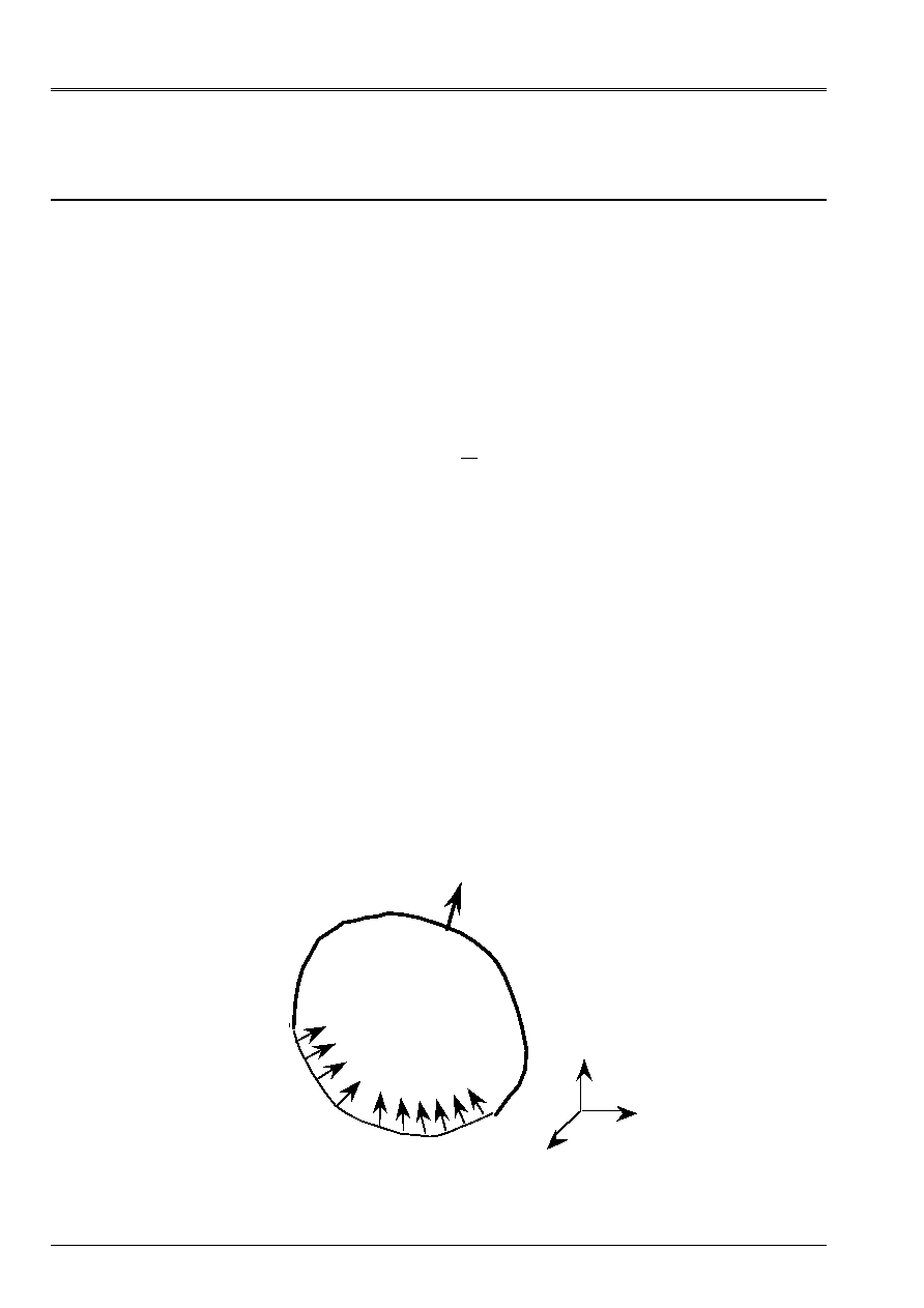
We represent on the figure [Figure 2.1-a] the unspecified confined field where the equation applies
of Helmholtz [éq 2.1-1] and conditions at the borders.
·
is open limited
R
3
of border
regular, partitionnée in
v
and
Z
;
=
v
Z
Fluid
Z
y
X
Border absorban
of impedance locali
N
Z
Z
v
V
N
Vibratory source
monochromatic
of normal amplitude
Appear 2.1-a: Configuration of the problem

Code_Aster
®
Version
3
Titrate:
Finite elements in accoustics
Date:
31/08/95
Author (S):
F. STIFKENS
Key:
R4.02.01-A
Page:
5/16
Manual of Reference
R4.02 booklet: Accoustics
HP-61/95/070/A
The equation [éq 2.1-1] is to be solved in a closed field
. Boundary conditions to take in
count on the border
field
express themselves in their most general form like:
p
p
+
=
N
éq 2.1-4
/N
appoint the operator of normal derivative.
,
are complex operators, who can be scalars, or integral operators
according to whether the border of application of the boundary condition is with local reaction or reaction not
local (case of the interaction fluid-structure).
The developments currently carried out in Code_Aster relate to only conditions
with the limit with local reaction, for which
,
are scalars; the cases spécifiables are
the following:
·
=
0
0
0
,
,
who indicates a border of the field at imposed vibratory speed. In
effect, there exists a relation connecting the acoustic gradient of pressure complexes at the speed
vibratory particulate complex.
p
N
J
V
N
= -
0
éq 2.1-5
0
indicate the density of the fluid considered, and one imposes
V
N
, vibratory speed
normal with the wall (
V
N
=
v N
.
where
N
indicate the unit vector of the normal external with
border
).
·
=
0
0
0
,
,
relate to a border with acoustic impedance
Z
imposed.
Acoustic impedance
Z
is defined like the report/ratio of the pressure at the vibratory speed
particulate in the vicinity of the wall with imposed impedance:
Z
V
N
=
p
éq 2.1-6
·
=
0
0
0
,
,
represent the case where the acoustic pressure is imposed
p
with one
border (generally
=
0
, corresponding to
p
=
0
).

Code_Aster
®
Version
3
Titrate:
Finite elements in accoustics
Date:
31/08/95
Author (S):
F. STIFKENS
Key:
R4.02.01-A
Page:
6/16
Manual of Reference
R4.02 booklet: Accoustics
HP-61/95/070/A
3
Conventional formulation in pressure
3.1
Mathematical expression of the problem
The standard procedure aiming at posing the problem with the conventional finite elements is as follows:
·
the sufficiently regular solution of the problem is supposed,
()
p
H
2
. One multiplies
the equation:
(
)
+
=
K
2
0
p
éq 3.1-1
by a function test
.
One integrates on
and one uses the formula of Green. The border
field
, subdivides itself in 2 areas, an area at imposed vibratory speed,
v
and one
area with imposed acoustic impedance,
Z
. The equation obtained can be rewritten under
form:
()
()
grad
grad
p.
p.
p.
.
-
+
+
=
2
2
0
0
0
C
FD
J
Z
dS
J
V
dS
Z
v
N
éq 3.1-2
·
FD
represent an element of differential volume in
and
dS
represent an element of
surface on
.
·
particulate vibratory speed is then determined by:
()
v
grad
=
J
0
p
éq 3.1-3
3.2
Discretization by finite elements
In the case of the conventional finite elements, the elementary integrals are four
K MR. C U
E
E
E
E
,
,
,
according to the decomposition indicated in [éq 3.2-3] (
K
E
is the matrix of rigidity,
M
E
the matrix of mass,
C
E
the matrix of damping and
U
E
the vector source). Two of them
come from voluminal integrals, the two others are the result of integrals respectively on
a vibrating surface and on a surface with imposed impedance.
It will be supposed that the total co-ordinates of an element can be written thanks to the data of
m
elementary functions of form
H
I
:
OM
OM
=
=
H
I
I
I
m
1
éq 3.2-1
One is given moreover, of the basic functions
NR
I
, to describe the elementary pressure.

Code_Aster
®
Version
3
Titrate:
Finite elements in accoustics
Date:
31/08/95
Author (S):
F. STIFKENS
Key:
R4.02.01-A
Page:
7/16
Manual of Reference
R4.02 booklet: Accoustics
HP-61/95/070/A
The pressure inside an element will be able to be written:
(
)
(
)
p
,
NR
,
I
E
I
m
IE
X y Z
P
=
=
1
éq 3.2-2
where
P
IE
is the pressure with the node
I
element
E
.
In the case of isoparametric finite elements, basic functions
NR
I
are equal to the functions
of form
H
I
.
On each element of the field, the problem with the finite elements in pressure is written:
(
) ()
()
K
M
C
P
U
E
E
E
E
E
J
Q
Q
Q
J
Q
-
+
= -
2
1
1
éq 3.2-3
where
()
P
E
q1
is the matrix column of the nodal values of the pressure on the element.
3.2.1 The matrix of rigidity
The matrix of rigidity
K
E
corresponds to the calculation of:
()
()
E
FD
grad
grad
p.
It admits like general term:
K
FD
ije
E
=
NR
NR
I
J
éq 3.2.1-1
3.2.2 The matrix of mass
The matrix of mass
M
E
corresponds to the calculation of:
1
2
C
FD
E
p.
It admits like general term:
M
C
FD
ije
E
=
1
2
NR NR
I
J
éq 3.2.2-1
3.2.3 The matrix of damping
The matrix of damping
C
E
corresponds to the calculation of:
0
Z
dS
Z
E
p.
It admits like general term:
C
Z
dS
ije
Z
E
=
0
NR NR
I
J
éq 3.2.3-1

Code_Aster
®
Version
3
Titrate:
Finite elements in accoustics
Date:
31/08/95
Author (S):
F. STIFKENS
Key:
R4.02.01-A
Page:
8/16
Manual of Reference
R4.02 booklet: Accoustics
HP-61/95/070/A
3.2.4 The vector source
The vector source
U
E
corresponds to the calculation of:
v
E
V
dS
N
0
It admits like general term:
U
V
dS
IE
N
v
E
=
0
NR
I
éq 3.2.4-1

Code_Aster
®
Version
3
Titrate:
Finite elements in accoustics
Date:
31/08/95
Author (S):
F. STIFKENS
Key:
R4.02.01-A
Page:
9/16
Manual of Reference
R4.02 booklet: Accoustics
HP-61/95/070/A
4
Mixed formulation pressure-speed
4.1
Mathematical expression of the problem
4.1.1 Formulation
local
The equation of Helmholtz [éq 1-1] with the boundary conditions [éq 2.1-3] result in fact from
local equations below:
I
I
Z
V
Z
N
v
p div
p
.
p
.
+
=
+
=
=
=
-
-
-
-
v
v grad
v N
v N
0
0
1
0
in
in
on
on
éq 4.1.1 1
éq 4.1.1 2
éq 4.1.1 3
éq 4.1.1 4
where
=
1
0 2
/
C
is the adiabatic coefficient of compressibility of the fluid.
The mathematical problem is as follows: being given functions
(
)
Z
L
Z
and
(
)
V
N
V
H
1
2
, to find functions
p
and
v
defined in
and with values in
C
checking these
equations. They describe, in harmonic mode of pulsation
, small fluctuations in pressure
p
and speed
v
starting from the at-rest state (c.à.d. acoustic pressure and particulate speed
accoustics) of a fluid compressible homogeneous, isotropic, nonviscous, confined in
and subjected to
a distribution of normal velocity
V
N
on
V
.
0
,
and
C
the density, the coefficient of compressibility represent respectively
adiabat and the speed of sound relating to the fluid, in acoustic absence of disturbance; the coefficient
=
1/Z
is the localized admittance of constituent material
V
with the pulsation considered.
To build a method of approximation by finite elements of this problem, it is necessary of
to put in a variational form.
4.1.2 Mixed variational formulation
One takes the scalar product of the equation [éq 4.1.1-1] in
()
L
2
with an unspecified function
Q
in
()
H
1
(it is the function-test).
The formula of Green and the fact that
v
check the boundary conditions [éq 4.1.1-3] and [éq 4.1.1-4] us
allow to lead to:
+
-
= -
I
V
Z
v
N
pq *
pq *
.
Q *
Q *
v grad
éq 4.1.2-1
One proceeds in the same way with the equation [éq 4.1.1-1] by taking his scalar product in
()
L
2
with
a function-test
U
unspecified in
()
(
)
L
2
3
one obtains:
+
=
I
0
0
v U
grad U
. *
p. *
éq 4.1.2-2
Code_Aster
®
Version
3
Titrate:
Finite elements in accoustics
Date:
31/08/95
Author (S):
F. STIFKENS
Key:
R4.02.01-A
Page:
10/16
Manual of Reference
R4.02 booklet: Accoustics
HP-61/95/070/A
Now we multiply [éq 4.1.2-1] by
J
0
and [éq 4.1.2-2] by
-
J
0
, then we do it
change of function:
J
v
v
!
Thus we obtain the mixed variational formulation [éq 4.1.2-3]:
To find
()
p, v
×
X
M
such as:
-
-
+
= -
+
=
0
2
2
0
0
02
0
1
0
v grad
v U
grad U
U
.
Q *
/
pq *
pq *
Q *
Q
. *
. *
C
J
J
V
X
p
M
V
Z
N
éq 4.1.2-3
where:
()
()
()
{
}
X
X
I
I
=
=
=
H
L
L
1
2
2
1 2 3
p
; p/
,
and:
()
(
)
()
()
{
}
M
I
I
I
=
=
=
=
L
L
2
3
2
1 2 3
v
v
; v
4.2
Discretization by finite elements.
The field
and its borders
V
and
Z
are cut out in fields and borders
elementary:
E
eV
eZ
,
,
on which are calculated elementary integrals.
To represent the fields of
p
E
and of
v
E
inside the element one uses the same functions
basic
NR
I
.
Inside each element (comprising m nodes) one writes:
(
)
(
)
(
)
OM
OM
v
v
E
I
m
IE
E
I
m
IE
E
I
m
IE
p
=
=
=
=
=
=
NR
,
p
NR
,
NR
,
I
I
I
1
1
1
,
are the curvilinear co-ordinates of a three-dimensional element;
OM
I
E
is the vector position of the node
M
I
element
E
with
m
nodes;
NR,
,
I
I
m
=
1
are the basic functions on the element
E
;
v
IE
“acceleration” with the node is the vector
M
I
element
E
.
Code_Aster
®
Version
3
Titrate:
Finite elements in accoustics
Date:
31/08/95
Author (S):
F. STIFKENS
Key:
R4.02.01-A
Page:
11/16
Manual of Reference
R4.02 booklet: Accoustics
HP-61/95/070/A
In this case the system of equations [éq 4.1.2-3] is written matriciellement for each element
E
:
p
Q
p
Q
J p
Q
J
Q
E E
E
E
E
E E
E
E
E
E E
E
E
E
E
E
E
v K U
v M U
v C U
S U
*
*
*
*
*
*
*
*
-
+
= -
2
éq 4.2-1
where:
{
}
p
p
statement
v
v
statement
v
v
E E
E
E
T
E
X
E
y
E
Z
E
m
E
MX
E
my
E
mz
E
v
v
= =
1
1
1
1
,
,
,
,
,
,
“
is the vector solution in
the element
E
;
4.2.1 The matrix of rigidity
K
E
is the matrix of elementary “rigidity”, corresponding to the calculation of the following part of
[éq 4.1.2-3]:
E
E
E
-
+ -
0
02
0
v grad
v U
grad U
.
Q *
. *
p. *
One can write it by breaking up it into
mxm
under matrices
K
ije
dimensions 4 X 4 like
below:
K
K
K
K
K
K
K
K
K
K
E
E
J
E
m
E
I
E
ij
E
im
E
m
E
mj
E
mm
E
I J
m
=
=
11
1
1
1
1
1
“
“
“
“
“
“
#
for
,
,
with the following terms for
K
ije
:
K
ije
I
J
I
J
I
J
J
I
I
J
J
I
I
J
J
I
I
J
X
y
Z
X
y
Z
E
E
E
E
E
E
E
E
E
=
-
-
-
-
-
-
0
0
0
0
0
0
0
0
0
0
0
02
0
02
0
02
NR NR
NR NR
NR NR
NR NR
NR NR
NR NR
NR NR
NR NR
NR NR

Code_Aster
®
Version
3
Titrate:
Finite elements in accoustics
Date:
31/08/95
Author (S):
F. STIFKENS
Key:
R4.02.01-A
Page:
12/16
Manual of Reference
R4.02 booklet: Accoustics
HP-61/95/070/A
4.2.2 The matrix of mass
M
E
is the matrix of elementary “mass”, corresponding to the calculation of:
1
2
/
pq *
C
Its coefficients are as follows:
M
C
I J
R
m
R
m
ije
I
J
=
=
-
-
1
1
4
3
4
3
1
2
/
NR NR
,
,
,
for
with
=,
#
#
#
The other terms are null
4.2.3 The matrix of damping
C
E
is the matrix of elementary “damping”, coming from calculation from:
Ve
0
pq *
Its coefficients are as follows:
C
I J
R
m
R
m
ije
I
J
Ve
=
=
-
-
0
1
4
3
4
3
1
NR NR
,
,
,
for
with
=,
#
#
#
The other terms are null.
4.2.4 The vector source
S
E
is the vector elementary “source”, representing the calculation of the terms
:
Z
E
V
N
0
Q *
Its components are as follows:
S
V
I J
R
m
R
m
IE
N
I
Z
E
=
=
-
-
0
1
4
3
4
3
1
NR
,
,
,
for
with
=,
#
#
#
The other terms are null.
After having obtained the field
p, v
on the field
by resolution of the equation [éq 4.2-1] assembled,
one returns to the field
p, v
by the opposite change of function; one can calculate the intensities
acoustics defined by [éq 1-1] which are in this case continuous in all the field
….

Code_Aster
®
Version
3
Titrate:
Finite elements in accoustics
Date:
31/08/95
Author (S):
F. STIFKENS
Key:
R4.02.01-A
Page:
13/16
Manual of Reference
R4.02 booklet: Accoustics
HP-61/95/070/A
5
Controls specific to acoustic modeling
At the time of a study by modeling in acoustic finite elements with Code_Aster one uses
general controls and of the controls which are specific to accoustics, or of which key words and
options are particular with this discipline; we present the list below of it.
Definition of the characteristics of the propagation mediums
It is necessary to give the density (actual value) and the celerity of propagation (value
complex); one uses for that the control:
DEFI_MATERIAU
with the following key words:
key word factor:
FLUID
key words:
RHO
(density
0
)
CELE_C
(celerity
C
)
Example:
air = DEFI_MATERIAU (FLUID: (
RHO: 1.3
CELE_C: IH 343. 0. ));
In this case
0
= 343. + j0.
Assignment of the model
It is obligatorily necessary to specify that it is about the “acoustic” phenomenon and to choose one of the 3
possible modelings of accoustics; the control is thus used:
AFFE_MODELE
with the following key words for which one specifies the values of assignment
possible:
key word:
PHENOMENON: “ACOUSTIC”
MODELING
:
“3D”
or
“PLANE”
or
“3d_MIXTE”
Example:
guide = AFFE_MODELE (MESH: mall
AFFE: (
ALL: “yes”
MODELING: “3d_mixte”
PHENOMENON: “acoustic”));
Boundary conditions
One must affect values normal vibratory speed per face (or edge into two-dimensional) to
meshs defining the borders sources, and also values of acoustic impedance per face (edge
into two-dimensional) with the meshs defining the borders in imposed impedance.

Code_Aster
®
Version
3
Titrate:
Finite elements in accoustics
Date:
31/08/95
Author (S):
F. STIFKENS
Key:
R4.02.01-A
Page:
14/16
Manual of Reference
R4.02 booklet: Accoustics
HP-61/95/070/A
One uses the control specific to accoustics:
AFFE_CHAR_ACOU
with the following key words:
key word:
MODEL
key word factor:
VITE_FACE
key word:
NET
GROUP_MA
VNOR
(normal vibratory speed
V
N
)
key word factor:
IMPE_FACE
key word:
NET
GROUP_MA
IMPE
(acoustic impedance
Z
)
key word factor:
PRES_IMPO
NODE
GROUP_NO
NEAR
(pressure
p
imposed on the nodes)
Example:
characou = AFFE_CHAR_ACOU (
MODEL: guide
VITE_FACE: (
GROUP_MA: input
VNOR: IH 0.0135 0. ));
In this case
V
N
= 0.0135 + j0.
Calculation of the elementary matrices
The various elementary matrices (rigidity, mass and damping) are calculated by options
specific. The control is employed:
CALC_MATR_ELEM
with the key word
OPTION
for which one specifies the possible values of assignment:
key words:
OPTION:
“RIGI_ACOU”
“MASS_ACOU”
“AMOR_ACOU”
Example:
matele_k = CALC_MATR_ELEM (
MODEL: guide
CHAM_MATER: chamat
OPTION: “rigi_acou”).
Note:
the assembled matrices can be obtained directly with the macro control
MACRO_MATR_ASSE
and same options.
Calculation of the elementary vector source
The elementary vector is calculated by a specific option; it is obligatorily necessary to indicate it
loading. The control is employed:
CALC_VECT_ELEM
with the key word
OPTION
for which one specifies the only value of assignment
possible:
key words:
OPTION:
“CHAR_ACOU”
key words:
CHARGE
Example:
vectelem = CALC_VECT_ELEM (
MODEL: guide
CHAM_MATER: chamat
OPTION: “char_acou”
CHARGE: characou);

Code_Aster
®
Version
3
Titrate:
Finite elements in accoustics
Date:
31/08/95
Author (S):
F. STIFKENS
Key:
R4.02.01-A
Page:
15/16
Manual of Reference
R4.02 booklet: Accoustics
HP-61/95/070/A
Calculation of the solution
After assembly of the elementary matrices and vector the harmonic solution can be calculated
directly with the control:
DYNA_LINE_HARM
Example:
presharm = DYNA_LINE_HARM (
MATR_MASS: matasm
MATR_RIGI: matask
MATR_AMOR: matasi
FREQ: F
EXCIT: (VECT_ASSE: vectass COEF_MULT:- 1.);
PUIS_PULS:1 PHAS_DEG:90.));
Postprocessings
From the result of the resolution of the matric transcription of the equations [éq 3.1-2] or
[éq 4.1.2-3], of the controls of postprocessing allow to obtain the nodal fields of sizes
following acoustics:
·
level
L
p
of acoustic pressure
P
in
dB L
P
p
:
log
.
=
-
20
2 0 10
10
5
·
real part of the acoustic pressure
·
imaginary part of the acoustic pressure
·
active acoustic intensity
[]
I
v
=
1
2 Re p *
·
reactive acoustic intensity
[]
J
v
=
1
2 Im p *
These fields are calculated by the use of the ordering of postprocessing
CALC_ELEM
(the concept
result is of the type
“ACOU_HARMO”
or
“MODE_ACOU”
):
CALC_ELEM
with the key words
RESULT
and
OPTION
for which one specifies the values of assignment
possible:
key word:
RESULT
key word:
OPTION:
“PRES_ELNO_DBEL”
(level of pressure in dB)
“PRES_ELNO_REEL”
(real part of the pressure)
“PRES_ELNO_IMAG”
(imaginary part of the pressure)
“INTE_ELNO_ACTI”
(intensity activates)
“INTE_ELNO_REAC”
(intensity reactivates)
Example:
&presharm = CALC_ELEM (
MODEL: guide
CHAM_MATER: chamat
RESULT: presharm
OPTION: “pres_elno_dbel”);

Code_Aster
®
Version
3
Titrate:
Finite elements in accoustics
Date:
31/08/95
Author (S):
F. STIFKENS
Key:
R4.02.01-A
Page:
16/16
Manual of Reference
R4.02 booklet: Accoustics
HP-61/95/070/A
6 Conclusion
Modules were thus integrated in Code_Aster, making it possible to make calculations of accoustics
interior in low frequencies for complex geometries by two methods: finite elements
conventional acoustics and mixed acoustic finite elements.
The two formulations were validated by comparison with the same analytical solution; cases tests
are presented in the manual of V7 validation under coding AHLV100.
As it was envisaged, the precision, with identical mesh, is higher in the mixed case; if one holds
count overall dimension memory this superiority is advantageous only if we want to obtain it
field of intensity: one should use the mixed E.F only in this case there.
7 Bibliography
[1]
A. BOUIZI: 'Implemented of a computer code of finite elements for processing of
the equation of Helmholtz in space clos' - Work of end of studies, E.C.L. 1986.
[2]
A. BOUIZI: “Spectral Analysis of the equation of Helmholtz.” - Report/ratio of DEA, Central School
from Lyon, 1986.
[3]
A. BOUIZI: 'Mixed Finite elements in stationary linear accoustics: Development of
code AIRMEF' - Acoustic department. DER - EDF. HE-24/88.02. 1988.
[4]
A. BOUIZI, Mr. COURTADE, D. JEANDEL, E. LUZZATO, A. MIGNOT, C. SURRY. :
'Conditions of compatibility of Brezzi-Babuska for methods finite elements mixed
in conformity in Mechanics and Acoustique' AUM, Acts of the 8th French Congress of
Mechanics, Nantes, 1987.
[5]
A. BOUIZI, Mr. COURTADE, D. JEANDEL, E. LUZZATO, C. SURRY: 'Processing of the equation
of Helmholtz by a code of mixed finite elements in space clos' GAMI, Conference Vibrations
Shocks, 1988, ECL, 1988.
[6]
A. BOUIZI: 'Resolution of the equations of linear Accoustics by a method of elements
stop mixtes'. Thesis presented in front of the Central School of Lyon - Speciality: Mechanics -.
Supported 02/03/89.
[7]
C. HABASQUE: 'Experimental Validation of the computer code of internal, Low accoustics
Fréquence'. Report/ratio of training course of DEA. ECL 1986 (+ Project of end of studies).
[8]
A. ADOBES: “Numerical and experimental Study of the fields of standing waves” Report/ratio
DER/EDF - HE-2287.22
[9]
F. STIFKENS, A. ADOBES: “Assessment of the integration of the conventional finite elements in Aster” -
Ratio DER/EDF - HP-64/91.149
[10]
F. STIFKENS: “Integration of the mixed acoustic finite elements in Aster” Ratio DER/
EDF - HP-61/92.081