
Code_Aster
®
Version
2.3
Titrate:
Elements vibroacoustic
Date:
02/11/92
Author (S):
Fe WAECKEL
Key:
R4.02.02-A
Page:
1/12
Manual of Reference
R4.02 booklet: Accoustics
HI-75/7952/A
Organization (S):
EDF/EP/AMV
Manual of Reference
R4.02 booklet: Accoustics
Document: R4.02.02
Vibroacoustic elements
Summary:
The elements described here make it possible to carry out calculations of the frequencies and clean modes of a structure
coupled to a fluid. They also allow the acoustic calculation of answer.
After the formulation of the problem of coupling fluid-structure, this document describes the step followed for
to implement in Aster the new finite elements.

Code_Aster
®
Version
2.3
Titrate:
Elements vibroacoustic
Date:
02/11/92
Author (S):
Fe WAECKEL
Key:
R4.02.02-A
Page:
2/12
Manual of Reference
R4.02 booklet: Accoustics
HI-75/7952/A
Contents
1 Introduction ............................................................................................................................................ 3
2 vibroacoustic coupling ................................................................................................................ 4
2.1 Presentation .................................................................................................................................... 4
2.2 Formulation of the vibroacoustic problem ..................................................................................... 4
2.2.1 Description of the structure ..................................................................................................... 4
2.2.1.1 Conservation equation of the momentum ........................................... 5
2.2.1.2 Relation of compatibility ............................................................................................ 5
2.2.1.3 Law of behavior in isotropic linear elasticity .................................................. 5
2.2.2 Description of the fluid ............................................................................................................... 5
2.2.2.1 Conservation equation of the momentum ........................................... 5
2.2.2.2 Conservation equation of the mass ...................................................................... 5
2.2.2.3 Law of behavior ................................................................................................. 6
2.2.2.4 Equation of propagation waves or equation of Helmholtz ................................ 6
2.2.3 Description of the interaction fluid-structure ............................................................................ 6
2.2.4 Formulation of the problem coupled ........................................................................................... 6
2.3 Variational equations associated the problem .......................................................................... 7
2.3.1 Variational equations associated the structure ................................................................ 7
2.3.2 Variational equation associated the equation of the fluid .......................................................... 7
2.4 Discretization by finite elements ..................................................................................................... 8
2.5 Choice of an additional variable for the description of the fluid ................................................. 8
2.5.1 Formulation of the new problem ........................................................................................ 8
2.5.2 Variational formulation associated the problem (P') ........................................................... 9
2.6 Discretization by finite elements ..................................................................................................... 9
2.7 Calculations of acoustic answer ..................................................................................................... 10
2.7.1 Speed imposed on the fluid .................................................................................................... 10
2.7.2 Impedance imposed on a wall of the fluid ........................................................................ 10
2.7.3 Discretization by finite elements .......................................................................................... 11
3 Integration in Aster ......................................................................................................................... 11
4 Bibliography ........................................................................................................................................ 12

Code_Aster
®
Version
2.3
Titrate:
Elements vibroacoustic
Date:
02/11/92
Author (S):
Fe WAECKEL
Key:
R4.02.02-A
Page:
3/12
Manual of Reference
R4.02 booklet: Accoustics
HI-75/7952/A
1 Introduction
The vibratory behavior of a structure is often modified if the aforementioned is in the presence of a fluid:
it is what is called the vibroacoustic coupling. One distinguishes the cases from coupling into two
categories: either the fluid is infinite (it is the case of the immersed structures), or the fluid is contained
in a limited medium (it is the case of the tanks more or less filled with fluid).
The finite elements described here make it possible to solve the problems of coupling with a fluid of
finished dimension.
General notations:
P
:
instantaneous total pressure in a point of the fluid,
p
0
:
pressure at rest,
p
:
acoustic pressure,
T
:
instantaneous total density in a point of the fluid,
0
:
density at rest,
:
acoustic density,
S
:
density of the structure,
X
:
acoustic displacement,
U
:
displacement of the structure,
:
gradient of acoustic displacements,
,
F
: pulsation, frequency,
C
:
speed of sound in the fluid,
,
K
:
wavelength, numbers wave,
:
tensor of the stresses of the structure,
:
tensor of the structural deformations,
C
:
tensor of elasticity of the structure,
T
:
tensor of the stresses of the fluid.
Code_Aster
®
Version
2.3
Titrate:
Elements vibroacoustic
Date:
02/11/92
Author (S):
Fe WAECKEL
Key:
R4.02.02-A
Page:
4/12
Manual of Reference
R4.02 booklet: Accoustics
HI-75/7952/A
2
Vibroacoustic coupling
2.1 Presentation
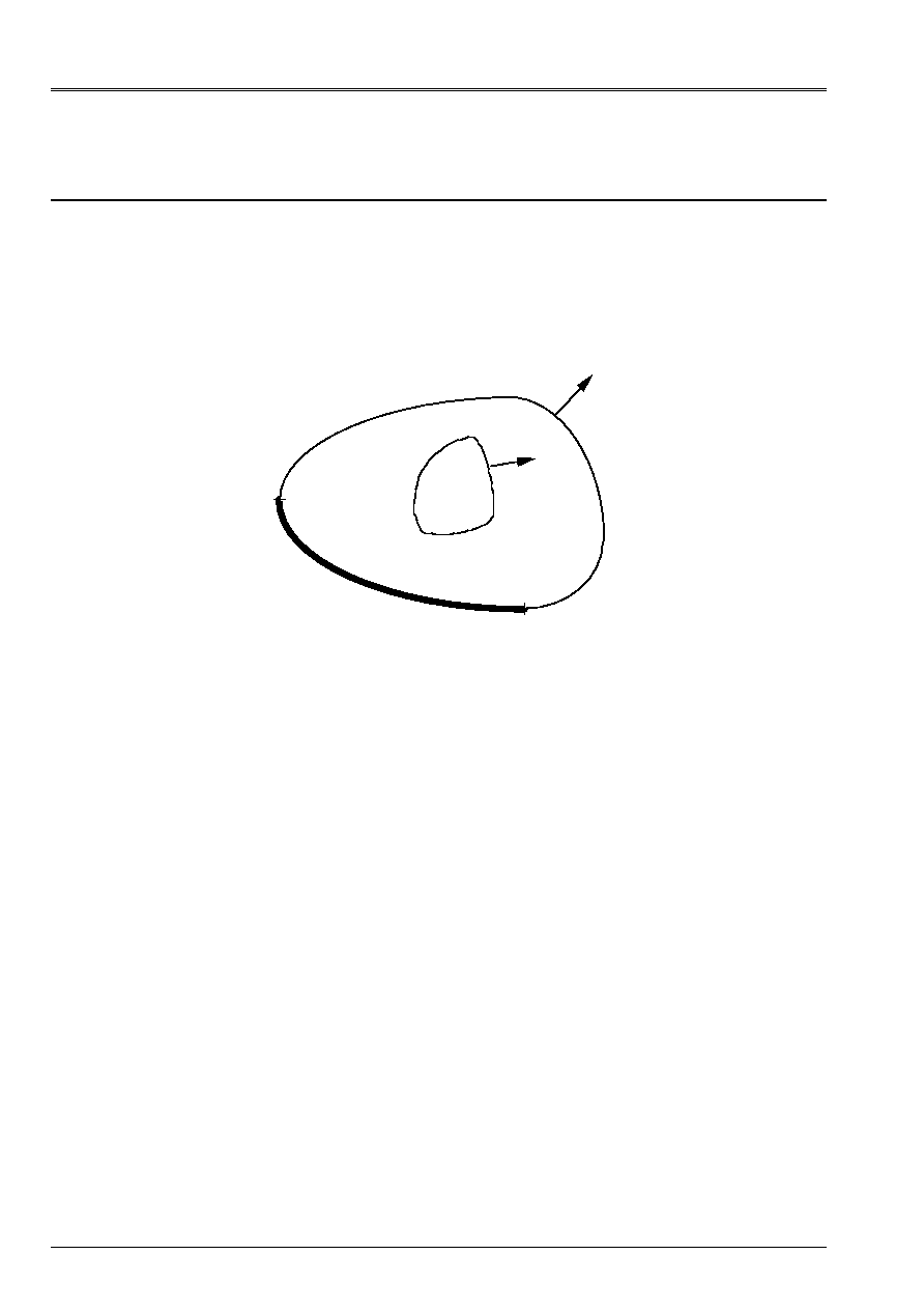
That is to say an elastic structure defined in a field
S
who vibrates in the presence of a true fluid, not
weighing, compressible, in isentropic evolution defined in a field
F
. One indicates by
=
F
S
,
their common surface.
One notes
N
, the normal external with the fluid field
F
.
Known
Sf
NS
S
N
F
At a given moment, the state of the fluid is defined by its field of pressure
P
and that of the structure by
its field of displacement
U
.
It is considered that the coupled system is subjected to small disturbances around its state
of balance where the fluid and the structure are at rest.
As follows:
P
=
p
0
+ p
U = U (U
0
= 0)
The problem of interaction fluid-structure then consists in solving two problems simultaneously:
·
one in the structure subjected, on
, with a field of pressure
p
imposed by the fluid
·
the other in the fluid subjected to a field of displacement
U
wall
.
2.2
Formulation of the vibroacoustic problem
2.2.1 Description of the structure
Assumption:
The structure is homogeneous and obeys the laws of linear elasticity.
Taking into account this assumption, one can write the various following equations controlling the state of
the structure [bib2].
Code_Aster
®
Version
2.3
Titrate:
Elements vibroacoustic
Date:
02/11/92
Author (S):
Fe WAECKEL
Key:
R4.02.02-A
Page:
5/12
Manual of Reference
R4.02 booklet: Accoustics
HI-75/7952/A
2.2.1.1 Conservation equation of the momentum
The conservation equation of the momentum is written, in the absence of voluminal forces
others that inertias:
ij, J
-
S
D
2
U
I
dt
2
= 0
[éq 2.2.1.1-1]
where:
S
is the density of the structure,
U
is displacement,
ij
is the tensor of the stresses.
2.2.1.2 Relation of compatibility
kl
= 1
2
U
K, L
+ U
L, K
[éq 2.2.1.2-1]
where
kl
is the tensor of the deformations
2.2.1.3 Law of behavior in isotropic linear elasticity
ij
= C
ijkl
kl
[éq 2.2.1.3-1]
with the moduli of elasticity
C
ijkl
checking the identities:
C
ijkl
=
C
klij
=
C
jikl
=
C
ijlk
C
being the tensor of elasticity.
2.2.2 Description of the fluid
Assumption: the fluid obeys the laws of linear accoustics.
Taking into account this assumption, the equations controlling the state of the fluid are:
2.2.2.1 Conservation equation of the momentum
The conservation equation of the momentum is written, in the absence of sources:
T
ij, J
-
0
D
2
X
I
dt
2
= 0
[éq 2.2.2.1-1]
where:
T
kl
is the tensor of the stresses in the fluid,
0
is the density of the fluid in a natural state,
X
is the field of displacement of a particle of fluid.
2.2.2.2 Conservation equation of the mass
With the first command and in the absence of acoustic sources, it is expressed by the relation:
p
T
0 div
X
T
0
+
=
[éq 2.2.2.2-1]
Code_Aster
®
Version
2.3
Titrate:
Elements vibroacoustic
Date:
02/11/92
Author (S):
Fe WAECKEL
Key:
R4.02.02-A
Page:
6/12
Manual of Reference
R4.02 booklet: Accoustics
HI-75/7952/A
2.2.2.3 Law of behavior
T
ij
= - p
ij
[éq 2.2.2.3-1]
The fluid is supposed in evolution barotrope (the pressure
p
is, for the fluid given, a function
known only density)
p
C
=
02
;
where
C
0
is the speed of sound in the fluid at rest.
2.2.2.4 Equation of propagation waves or equation of Helmholtz
One deduces it by combination from the conservation equations from the mass [éq 2.2.2.2-1] and from
momentum [éq 2.2.2.1-1] written in harmonic mode, with the pulsation
:
p + K
2
p = 0
[éq 2.2.2.4-1]
where
K
=
/
C
is the number of wave.
2.2.3 Description of the interaction fluid-structure
With the interface fluid-structure (
), the fluid being nonviscous, it does not adhere to the wall. One thus writes:
·
the continuity of the normal stresses:
ij
.n
I
= T
ij
.n
I
= - p
ij
.n
I
[éq 2.2.3-1]
·
the continuity normal speeds:
I
dt
.n
I
= dx
I
dt
.n
I
[éq 2.2.3-2]
2.2.4 Formulation of the coupled problem
Ultimately, the formulation of the problem of vibroacoustic in terms of displacements for
structure and of pressure in the fluid led to the equations of the harmonic problem (
P
):
C
ijkl
.u
K, lj
+
2
S
U
I
= 0
in
S
[éq 2.2.4-1]
p + K
2
p = 0
in
F
C
ijkl
.u
K, L
.n
I
= - p
ij
.n
I
on
U N
p
N
I
I
.
=
1
0
2
on
Code_Aster
®
Version
2.3
Titrate:
Elements vibroacoustic
Date:
02/11/92
Author (S):
Fe WAECKEL
Key:
R4.02.02-A
Page:
7/12
Manual of Reference
R4.02 booklet: Accoustics
HI-75/7952/A
2.3
Variational equations associated the problem
One solves the problem coupled by using the finite element method starting from the weak formulation
problem.
2.3.1 Variational equations associated the structure
That is to say
U
, kinematically acceptable in
S
, the equation [éq 2.2.4-1] can be written in the form
integral:
S
C
ijkl
.u
K, Li
U
I
+
2
S
U
I
U
I
FD = 0
After integration by part, one obtains the weak formulation:
S
C
ijkl
.u
K, L
U
I, J
-
2
S
U
I
U
I
FD -
C
ijkl
U
I
U
K, L
.n
I
S
dS = 0
Maybe, if one takes into account the boundary condition [eq 2.2.3 - 1]:
S
C
ijkl
.u
K, L
U
I, J
-
2
S
U
I
U
I
FD -
p
U
I
.n
I
dS = 0
[éq 2.3.1-1]
2.3.2 Variational equation associated the equation of the fluid
That is to say
p
, kinematically acceptable in
F
. One writes in variational form the equation
[éq 2.2.2.4-1]:
F
p
p + K
2
p
p FD = 0
(
)
-
+
=
-
+
=
div p p FD
p
p FD
K
p p FD
p dpn ds
p
p FD
K
p p FD
F
F
F
F
F
F
.
.
.
.
2
2
0
0
Maybe, if one takes into account the boundary condition [éq 2.2.3-1]
1
0
2
F
p.
p - K
2
p.
p FD -
U
N
.
p dS = 0
[éq 2.3.2-1]
Code_Aster
®
Version
2.3
Titrate:
Elements vibroacoustic
Date:
02/11/92
Author (S):
Fe WAECKEL
Key:
R4.02.02-A
Page:
8/12
Manual of Reference
R4.02 booklet: Accoustics
HI-75/7952/A
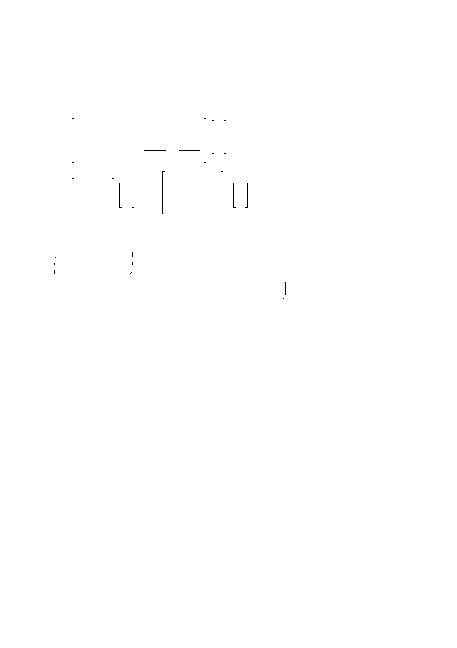
2.4
Discretization by finite elements
The approximation by finished parts of the complete problem leads then to the system:
K
2
M
- C
- C
T
H
0
.
2
-
Q
0
.c
2
U
p
= 0
maybe,
K
- C
0
H
U
p -
2
M
0
0
.C
T
Q
C
2
U
p = 0
where:
K
and
M
are the matrices of stiffness and mass of the structure,
H
and
Q
are the fluid matrices obtained respectively starting from the bilinear forms:
F
p.
p FD
and
p.
p FD
F
C
is the matrix of coupling obtained starting from the bilinear form
F
p. U
N
dS
The choice of the formulation led to a nonsymmetrical system matric what does not make it possible to use
conventional algorithms of resolution.
2.5
Choice of an additional variable for the description of the fluid
2.5.1 Formulation of the new problem
To obtain a symmetrical problem, one associates the variable pressure, a variable
additional. This new variable is, that is to say the potential of displacement of the fluid
such as
X
=
grad
[bib1], [bib4], [bib5], that is to say the variable
[bib3] such as
= -
.
. The variable
allows to take
in account directly fluids with variable density. However, it does not represent anything
physically. This is why, the potential of displacements is preferred to him.
One thus replaces displacement X of the fluid by grad
in the equations of the problem (
P
) [§ 2.2.4].
One thus obtains the new problem to be solved (
P
'):
C
ijkl
.u
K, lj
+
2
S
U
I
= 0
in
S
0
2
+ K
2
p = 0
in
F
[éq 2.5.1-1]
p =
0
2
in
F
[éq 2.5.1-2]
C
ijkl
.u
K, L
.n
I
= -
0
2
ij
.n
I
on
[éq 2.5.1-3]
U N
N
I
I
.
=
on
[éq 2.5.1-4]
Code_Aster
®
Version
2.3
Titrate:
Elements vibroacoustic
Date:
02/11/92
Author (S):
Fe WAECKEL
Key:
R4.02.02-A
Page:
9/12
Manual of Reference
R4.02 booklet: Accoustics
HI-75/7952/A
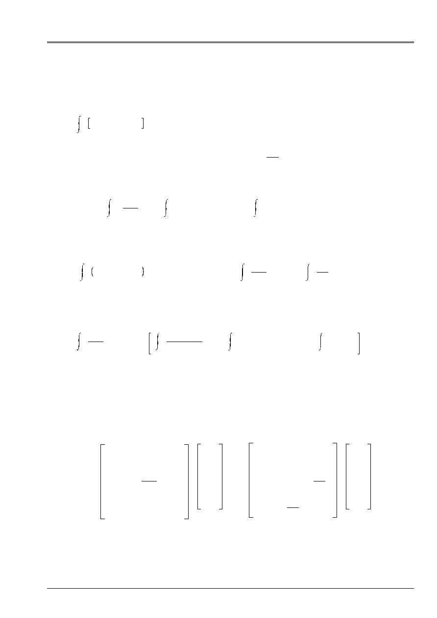
2.5.2 Variational formulation associated the problem (P')
One applies to the equation [éq 2.5.1-1] the formula of GREEN:
F
0
2
+ K
2
p
FD = 0
a.c.
[
]
-
+
=
K p
FD
N ds
F
F
2
0
2
0
2
0
grad
grad
a.c.
Maybe, if one takes into account the boundary condition [éq 2.5.1-3]
F
p
0
C
2
FD -
F
grad
grad
FD +
U
N
dS = 0
a.c.
[éq 2.5.2 - 1]
Moreover, one writes in weak form the equation [éq 2.5.1 - 2] for
Q
a.c.,
F
p -
0
2
Q FD = 0
Q a.c.
F
pq
0
C
2
FD -
2
F
Q
C
2
FD = 0
[éq 2.5.2 - 2]
By summoning the equations [éq 2.5.2 - 1] and [éq 2.5.2 - 2], one obtains the associated variational equation
with the fluid:
F
pq
0
C
2
FD -
0
2
F
Q + p
0
C
2
FD -
F
grad
grad
FD +
.u
N
dS = 0
(Q,
) a.c.
[éq 2.5.2 - 3]
2.6
Discretization by finite elements
While proceeding with the same step as that used in [§ 2.3], one is led to the system
matric according to:
K
O
0
0
M
F
0
C
2
0
0
0
0
U
p
-
2
M
0
0
.M
0
0
M
fl
C
2
0
.M
T
M
fl
T
C
2
0
.H
U
p
= 0
Code_Aster
®
Version
2.3
Titrate:
Elements vibroacoustic
Date:
02/11/92
Author (S):
Fe WAECKEL
Key:
R4.02.02-A
Page:
10/12
Manual of Reference
R4.02 booklet: Accoustics
HI-75/7952/A
K
and
M
being respectively matrices of stiffness and mass of the structure,
M
being the matrix of coupling fluid-structure obtained starting from the bilinear form:
U dS
and
M
F
,
M
fl
,
H
being fluid matrices, respectively obtained starting from the bilinear forms:
F
p
2
FD,
F
p
FD and of
F
grad
2
FD
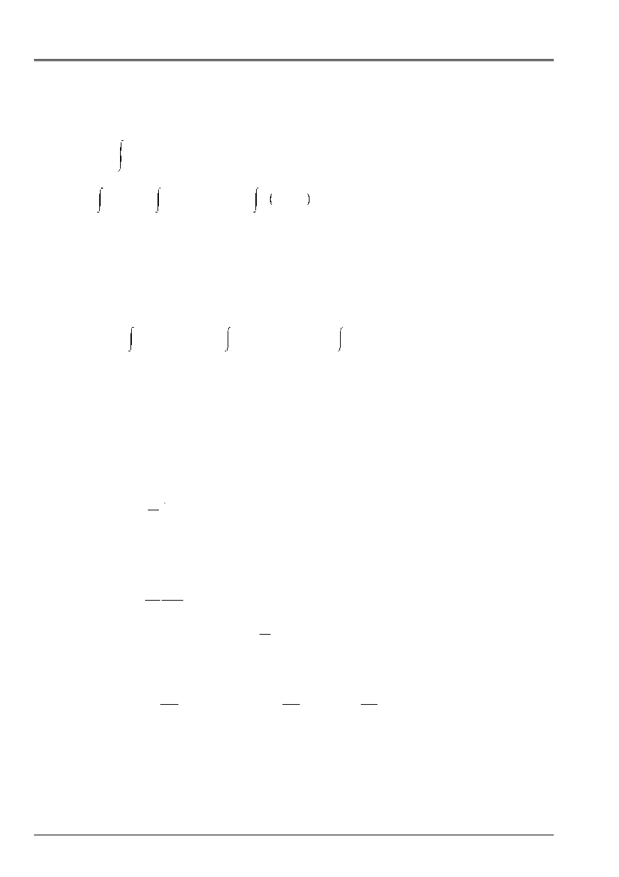
2.7
Calculations of acoustic answer
2.7.1 Speed imposed on the fluid
On a part
v
fluid border
F
, one can impose a limiting condition of normal speed type
v
0
.
The term of edge of the fluid is written then:
-
0
2
F
.u
N
dS =
-
0
2
F
-
v
.u
N
dS + I
0
v
v
0
dS
2.7.2 Impedance imposed on a wall of the fluid
On a part
Z
fluid border
F
, one can impose a limiting condition of impedance type
Z
.
p = Z v
N
where
vn
is the outgoing normal speed of the fluid.
By deferring this condition in the equation translating the conservation of the momentum
[éq 2.2.2.1 - 1] and by taking account of the law of behavior of the fluid [éq 2.2.2.3 - 1], one a:
grad
p +
0
Z
p = 0
[éq 2.7.2 - 1]
To preserve the symmetry of the system, one expresses the equation [eq 2.7.2 - 1] according to the potential of
displacement of the fluid
, one a:
grad
!!
+
=
0
3
3
0
Z
T
Maybe, in harmonic:
grad
+ I
0
Z
= 0
The term of edge of the fluid is written then:
0
2
0
2
3
02
.
.
N ds
N ds I
Z
ds
v
F
Z
F
=
+
-
Ultimately, to impose an impedance on a wall of the fluid amounts introducing into the system one
term of damping.
Code_Aster
®
Version
2.3
Titrate:
Elements vibroacoustic
Date:
02/11/92
Author (S):
Fe WAECKEL
Key:
R4.02.02-A
Page:
11/12
Manual of Reference
R4.02 booklet: Accoustics
HI-75/7952/A
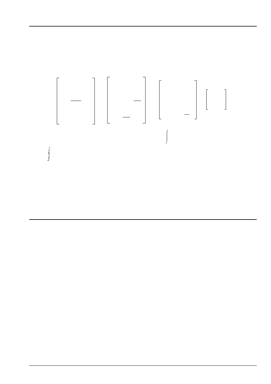
2.7.3 Discretization by finite elements
If one imposes limiting conditions of imposed speed type or impedance of wall imposed on the fluid,
one is led to solve the following matric system:
K
0
0
0
M
F
0
.
C
2
0
0
0
0
-
2
M
0
0
.
M
S
0
0
M
fl
C
2
0
.
M
S
T
M
fl
T
C
2
0
.
H
- I
3
0
0
0
0
0
0
0
0
0
2
Z
Q
=
0
I
V
0
Q being the matrix obtained starting from the bilinear form:
Z
2
dS
and
V
, the vector obtained from
v
0
v
0
dS
.
3 Integration
in
Aster
The elements described previously belong, for the fluid part, with modeling
“3d_FLUIDE”
phenomenon
MECHANICS
and, for the interface fluid-structure, with modeling
“FLUI_STRU”
same phenomenon.
They lead to voluminal or surface elements, for the fluid part, in pressure-potential of
displacement and with surface elements for the interface fluid-structure in potential of
displacement of the fluid-displacement of the structure.

Code_Aster
®
Version
2.3
Titrate:
Elements vibroacoustic
Date:
02/11/92
Author (S):
Fe WAECKEL
Key:
R4.02.02-A
Page:
12/12
Manual of Reference
R4.02 booklet: Accoustics
HI-75/7952/A
4 Bibliography
[1]
T. BALANNEC, S. COURTIER-ARNOUX, E. LUZZATO, P. THOMAS: Confrontation of tools
numerical of department AMV on a test of coupling fluid-structure. Internal report
E.D.F. D.E.R. HP-61/91.012
[2]
P. GERMAIN: Introduction to the mechanics of the continuous mediums. Masson
[3]
R.J. GIBERT: Vibrations of the structures. Interactions with the fluids. Sources of excitation
random. Collection of the Management of the Studies and Search for E.D.F. n°69.
[4]
R. OHAYON, R. VALID: True symmetric formulations off free vibrations off fluid-structure
interaction. Applications and extensions. International conference one numerical method for
coupled systems
[5]
P. THOMAS: Formulation of coupling fluid-structure for the modal analysis in SIVA.
Application to the three-dimensional elements. Internal report E.D.F.D.E.R. HP-35.82/259