Method multifrontale

Code_Aster

Version

5.0

Titrate:

Method multifrontale

Date:

26/02/01

Author (S):

C. ROSE

Key:

R6.02.02-B

Page:

1/18

Manual of Reference

R6.06 booklet: Direct methods

HI-75/01/001/A

Organization (S):

EDF/MTI/MN

Manual of Reference
R6.02 booklet: Direct methods
Document: R6.02.02

Method multifrontale

Summary:

The method multifrontale is a direct method particularly adapted to the resolution of the systems
linear whose matrix is hollow. This method includes a preliminary phase of renumerotation
intended to minimize the filling of the matrix during factorization.

This phase also makes it possible to gather the variables in “super-variables” or “super-nodes”. Factorization,
as for it, is carried out in the form of a continuation of elimination of super-nodes, in full matrices.
These full matrices allow the use of routines optimized like the BLAS, which obtain them
better performances on vectorial or scalar machines.

Having the factorized matrix, each resolution of system will require nothing any more but one
“gone up descent/” inexpensive.

Code_Aster

Version

5.0

Titrate:

Method multifrontale

Date:

26/02/01

Author (S):

C. ROSE

Key:

R6.02.02-B

Page:

2/18

Manual of Reference

R6.06 booklet: Direct methods

HI-75/01/001/A

Contents

1 Description of the method ..................................................................................................................... 3

1.1 Method LDLT for the full matrices ........................................................................................ 3

1.2 Hollow matrix and filling ........................................................................................................ 6

1.3 Method multifrontale ...................................................................................................................... 7

1.4 Descent - Increase ................................................................................................................... 13

2 Establishment and use in Code_Aster ..................................................................................... 14

3 Bibliography ........................................................................................................................................ 16

Appendix 1 Reference material of the method “Approximate Minimum dismantles” ................... 17

Appendix 2 Reference material Mongrel ......................................................................................... 17

Code_Aster

Version

5.0

Titrate:

Method multifrontale

Date:

26/02/01

Author (S):

C. ROSE

Key:

R6.02.02-B

Page:

3/18

Manual of Reference

R6.06 booklet: Direct methods

HI-75/01/001/A

Description of the method

The method multifrontale is a direct method of resolution of linear systems, which is
particularly adapted to the systems having a hollow matrix. It factorizes matrices
symmetrical or not, not necessarily definite positive. In the most general case, the method
multifrontale calls upon the method of Gauss with search for pivots.

The method established in Code_Aster is limited to the symmetrical matrices, and uses the algorithm

known as “

LDL

“, without search for pivot.

The resolution of a linear system is carried out in three stages:

renumerotation of the unknown factors,

factorization of the matrix,

gone up descent/.

If several linear systems, of the same matrix, are to be solved, only them
gone up descents/are to be carried out. The same if several of the same matrices structure are with
to factorize, the renumerotation of the unknown factors will not be to remake. This preliminary phase, which
the performance of factorization will ensure, has a considerable cost, however its relative weight (in
calculating time), decreases with the size of the matrices to factorize.

We will follow the following plan:

1) presentation of the method

LDL

conventional adapted to the full matrices. Concept

of elimination,

2) extension of the method to the hollow matrices, concept of filling,
3) presentation of the multi-frontal method.

1.1

Method LDLT for the full matrices

That is to say

With

, an invertible matrix, one knows that there is a lower triangular matrix

with diagonal

unit and a higher triangular matrix

, such as

With

L U

. The command of these matrices will be

With

is symmetrical, this decomposition can be written:

With

LDL

éq 1.1-1

where

is a diagonal matrix and

the matrix transposed of

, with diagonal unit.

Are

()

[]

I J

; from [éq 1.1-1] one deduces the expression from the coefficients from

and

. Indeed one

can write:

With

L D L

éq 1.1-2

being triangular lower than diagonal unit, and

diagonal, [éq 1.1-2] becomes:

()

With

L L

I J

min,

éq 1.1-3

Code_Aster

Version

5.0

Titrate:

Method multifrontale

Date:

26/02/01

Author (S):

C. ROSE

Key:

R6.02.02-B

Page:

4/18

Manual of Reference

R6.06 booklet: Direct methods

HI-75/01/001/A

There is to calculate the coefficients in many ways of

and

from [éq 1.1-3]. We go

to see the method called “by line” used usually in Code_Aster, and the method “by column”
used in the method multifrontale.

Method by line

Lines of

and

the ones after the others are calculated jointly. Let us suppose these lines

known until the command

(

)

, and also let us suppose that the coefficients of the line

are known

until the command

; [éq 1.1-3] is written, with

J I

With

L L

L D L

éq 1.1-4

One has as follows:

With

L L

éq 1.1-5

and in a similar way:

With

L L D

éq 1.1-6

With this method, each coefficient is calculated in only once (operation [éq 1.1-5]), while going
to seek the coefficients previously calculated, and by making the scalar product of

(

)

and

(

)

, with

L D

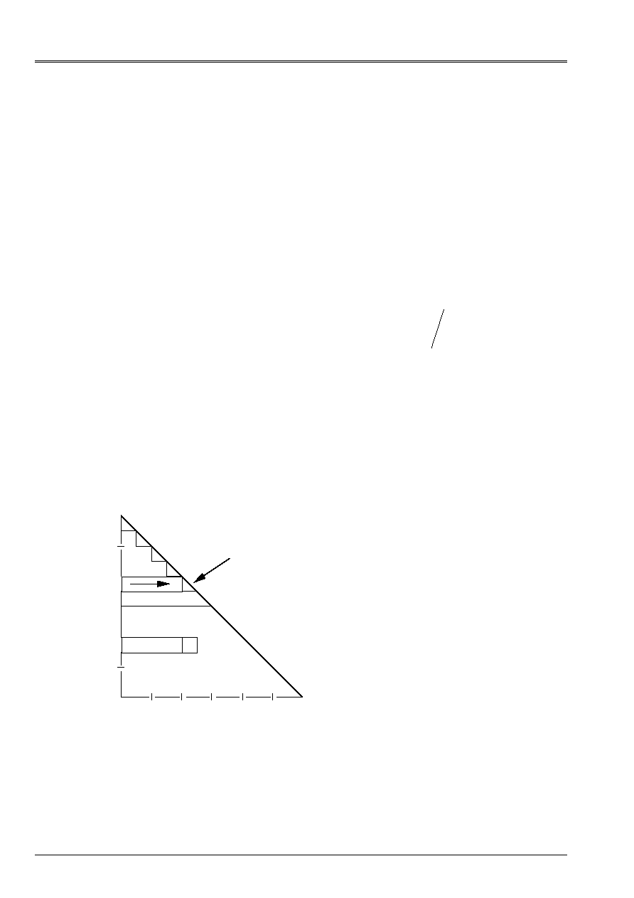
This algorithm is illustrated by [Figure 1.1-a].

(In gray and hatched, terms necessary

with the calculation of L

)

Appear 1.1-a

Code_Aster

Version

5.0

Titrate:

Method multifrontale

Date:

26/02/01

Author (S):

C. ROSE

Key:

R6.02.02-B

Page:

5/18

Manual of Reference

R6.06 booklet: Direct methods

HI-75/01/001/A

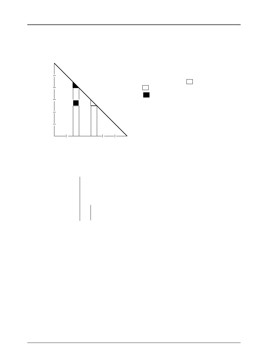
Method by columns
Let us examine the figure [Figure 1.1-b] following:

One adds to the column in

the column

, multiplied by the product of the terms

Appear 1.1-b

Let us suppose that the column

, i.e. terms

and

(

)

= +

, is known and

let us carry out the following algorithm:

(

)

for

to make

éq 1.1 - 7

for

to make

éq 1.1 - 8

= +,

saxpy

with

L D

with

L L D

= +

Let us make three note:

1) the operations [éq 1.1-7] are called the elimination of the unknown factor

. Indeed, after [éq 1.1-7],

one will make call under the column never again

in the continuation of the algorithm.

method by column is sometimes qualified of “looking forward method”; as soon as they are
calculated, the terms of the matrix act on the following terms. On the other hand, them
methods by line are called “looking backward methods”; one will seek the terms
previously calculated with each new calculation,

2) the operation [éq

1.1-7] is an operation of the type “saxpy”, one withdraws from the vector

(

)

= +

, the product of the constant

and of the vector

(

)

= +

3) having carried out [éq 1.1-7] for

fixed, let us see what it remains to do to know the column

()

+ +

is known (it easily is checked),

it is enough to divide the column

(

)

K J

= +

+ +

to have the value

final of the aforementioned.

Code_Aster

Version

5.0

Titrate:

Method multifrontale

Date:

26/02/01

Author (S):

C. ROSE

Key:

R6.02.02-B

Page:

6/18

Manual of Reference

R6.06 booklet: Direct methods

HI-75/01/001/A

(The terms above were wrongly confused

final and their name of programming which

contains the values of

modified during eliminations).

One thus deduces the general algorithm from it from factorization

LDL

by columns.

for

to make

for

to make

for

to make

= +,

for

/standardization/

elimination

saxpy

= +

with

L D

with

L L D

éq 1.1-9

Before passing to the concept of filling, it is advisable to make as of now a useful remark for
the continuation. If one looks at [éq 1.1-9], it appears that one can eliminate the unknown factor

, even if terms

(

)

= +

and

are not yet available. Indeed, it is enough to preserve the terms

(

)

L L D

, and to then add them under the terms

. These terms

(

)

L L D

varying

with

and

with

form a matrix associated with elimination with the unknown factor

, that one

will call thereafter the frontal matrix

1.2

Hollow matrix and filling

It is reminded the meeting that if the initial matrix comprises null terms, successive eliminations
cause filling, i.e. certain terms

are different from zero whereas it

initial term

With

is.

Let us suppose that before the elimination of the unknown factor

, the term

is null; if

and

are both

nonnull, [éq 1.1-9] shows that

also not no one will become him. This filling has an interpretation

graph. Let us suppose in this case that all the unknown factors are represented by the nodes of one
graph: the nodes will be connected

and

if and only if the term

With

matrix initial is nonnull.

With

is null with

connected to

and

connected to

, the elimination from the graphic point of view of

will consist in connecting then

and

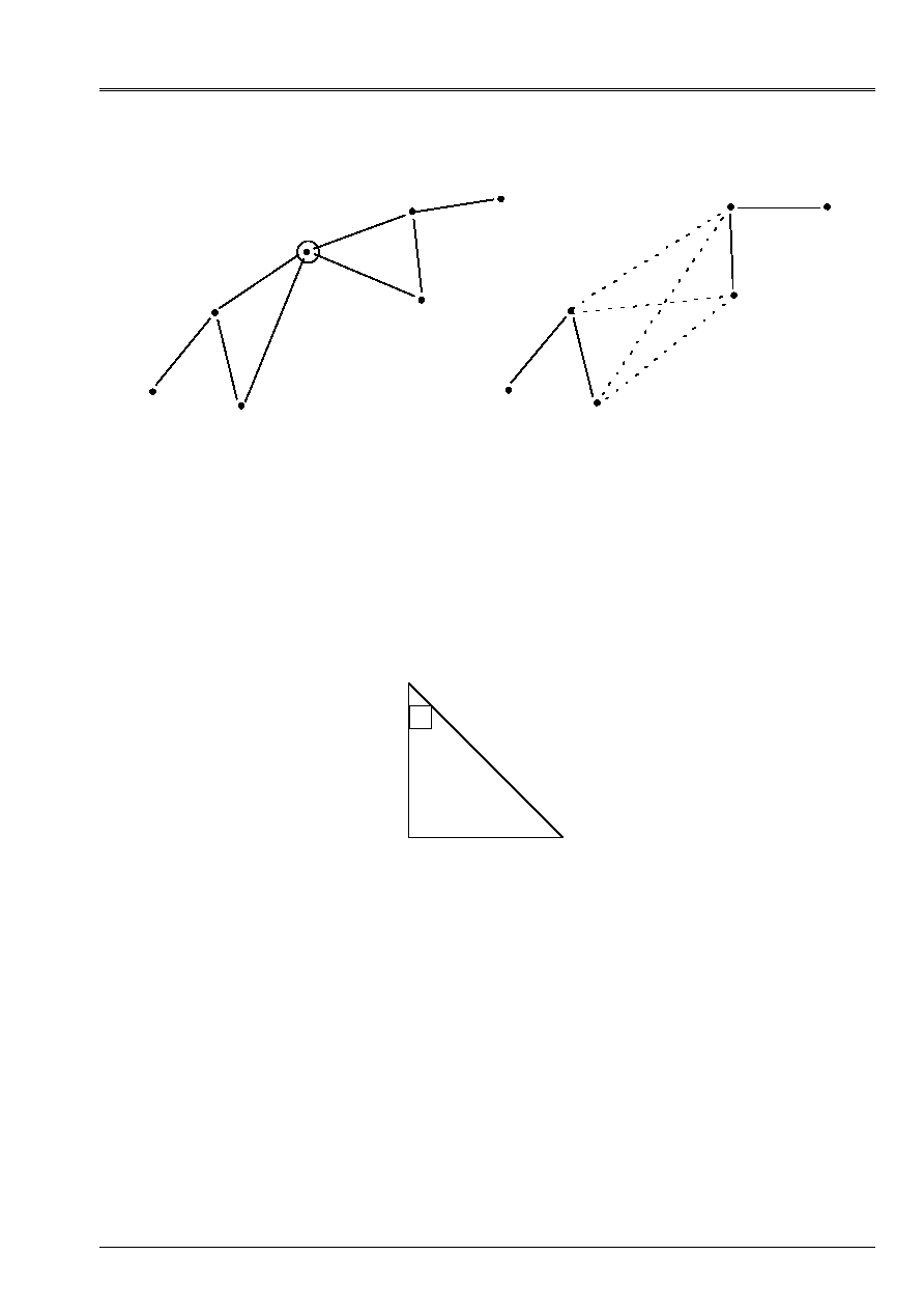
The figure [Figure 1.2-a] illustrates this interpretation. The edges in dotted line are those create by
the elimination of

. They correspond in the new nonnull terms of the matrix

Code_Aster

Version

5.0

Titrate:

Method multifrontale

Date:

26/02/01

Author (S):

C. ROSE

Key:

R6.02.02-B

Page:

7/18

Manual of Reference

R6.06 booklet: Direct methods

HI-75/01/001/A

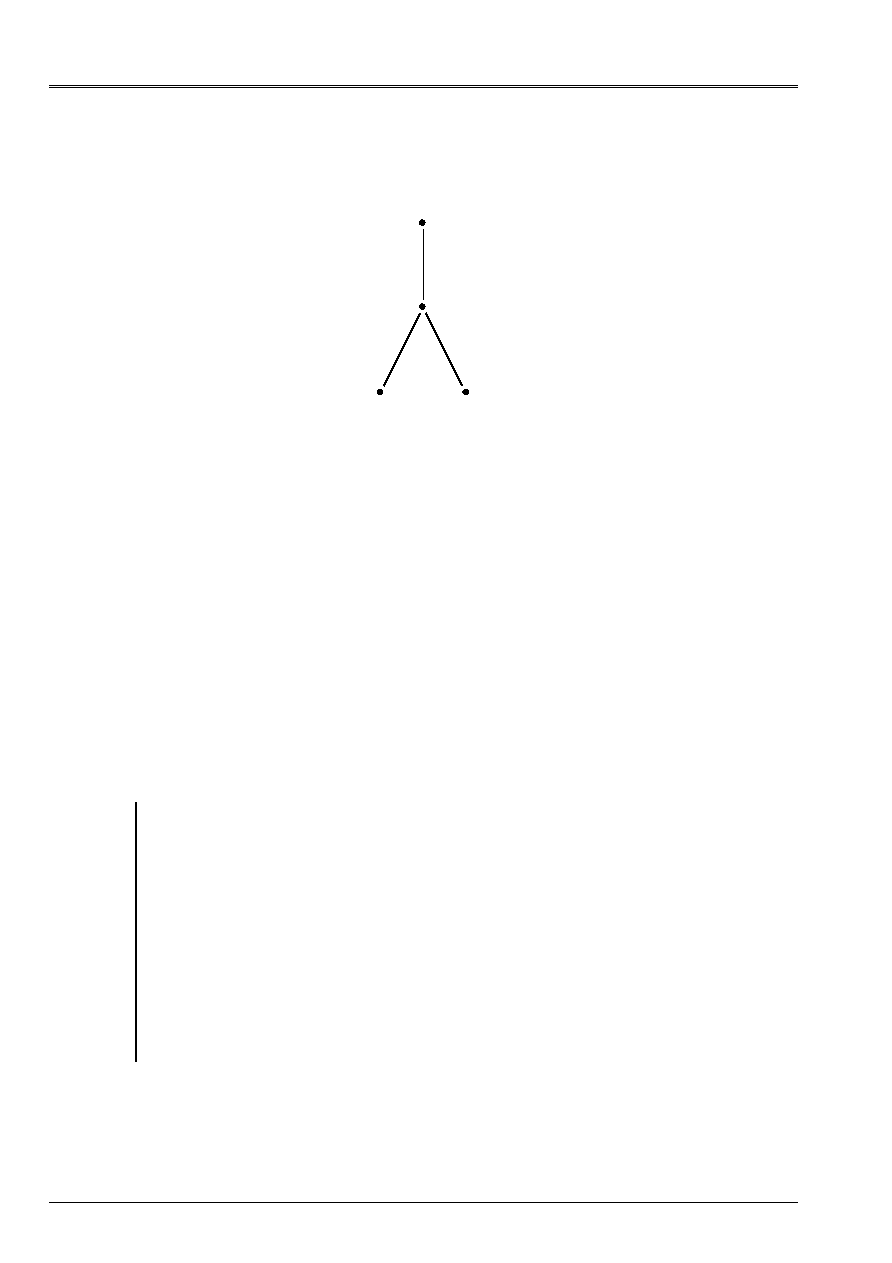
Appear 1.2-a: the elimination of the node J connects all its neighbors between them

1.3 Method

multifrontale

The method multifrontale is a direct method, of Gauss type, which aims at exploiting to the maximum it
hollow of the matrix to be factorized. It seeks, on the one hand, to minimize the filling by using one
optimal renumerotation, in addition, it extracts from the structure digs matrix information him
allowing to eliminate (cf page 5 notices (1)) unknown factors independently from/to each other.

Let us examine the simple case of the figure [Figure 1.3-a], where the matrix has only one null term,

With

Appear 1.3-a

Column 2 of

does not undergo the effects of the elimination of unknown factor 1, because the coefficient

With

then

(cf [éq 1.1-9] seen previously). Contributions to columns 3 and 4 of

, of unknown factors 1 and 2 are independent of their kind of elimination (it is necessary to look in detail

[éq 1.1-9]). Of this observation, one can introduce the concept of shaft of elimination presented by I. Duff
[bib1].

Code_Aster

Version

5.0

Titrate:

Method multifrontale

Date:

26/02/01

Author (S):

C. ROSE

Key:

R6.02.02-B

Page:

8/18

Manual of Reference

R6.06 booklet: Direct methods

HI-75/01/001/A

The shaft of elimination of the matrix

With

can be represented by the figure [Figure 1.3-b].

Appear 1.3-b

This tree structure contains two concepts:

the independence of certain eliminations (here variables 1 and 2), which will lead to one

possible parallelism of the operations,

the minimization of the operations to be carried out, (one sees on the tree structure that the term

is not

not to calculate).

Being given a hollow matrix, which one knows the filling, the shaft of elimination can be
built as follows:

all the sheets of the shaft (lower ends) correspond to the unknown factors

, such

that

With

for

with

. Here 1 is of course a sheet because there is no term

With

for

, 2 is also a sheet bus

With

one

node

has as a father

, if

is the smallest number of line such as

With

. Here, 3 is

the father of 1 and 2.

Note:

1) one employs starting from now the vocabulary of the shaft, graph theory, sheet,

node… Here the shaft is turned over, its sheets are in bottom,

2) one will refer to [bib1] for more details and the demonstrations of the validity of the method,
3) in the example above, the command of elimination between the unknown factors (3) and (4) is fixed by

initial classification, one could have permuted the lines and the columns of the matrix and to have 4
like father of 1 and 2,

4) it should be noticed that the manufacture of this tree structure must take into account the terms

nonnull obtained by filling during elimination. (One will see more details on it
subject in [bib2]). One cannot manufacture the shaft of elimination only starting from the matrix
dig initial: it is necessary to also know the terms of filling like already mentioned
previously. The numerical factorization of the method multifrontale is preceded by one
important phase: the simulation of eliminations and thus, the creation of the nonnull terms.
One calls also this simulation, logical elimination or symbolic system. This simulation takes place
during the first phase: the renumerotation. One will see the four phases of
method multifrontale, most important being the first and the fourth.

Code_Aster

Version

5.0

Titrate:

Method multifrontale

Date:

26/02/01

Author (S):

C. ROSE

Key:

R6.02.02-B

Page:

9/18

Manual of Reference

R6.06 booklet: Direct methods

HI-75/01/001/A

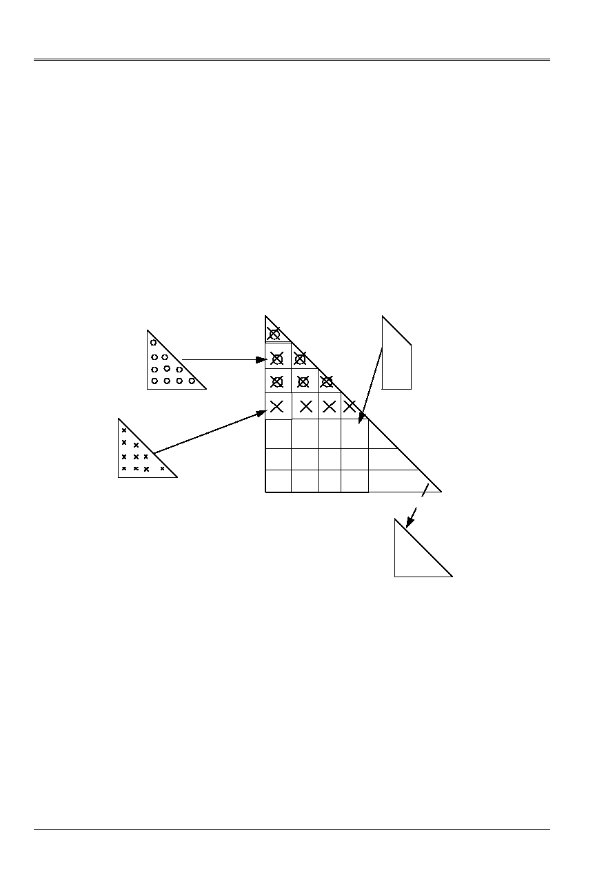
First phase: The renumerotation of the “minimum dismantles” (minimum degree).

The purpose of this renumerotation is first to minimize the number of operations to be carried out at the time of
factorization. For that one simulates the elimination of the nodes and one chooses like candidate for
elimination the node of the graph having the lowest number of neighbors. One uses the concept here of
graph seen with the figure [Figure 1.2-a]. The initial hollow matrix defines the graph on which one
work. This last is then updated to each elimination of nodes (creation of links).
simulation of the filling makes it possible to achieve the second goal which is the manufacture of the shaft
of elimination seen in the preceding paragraph. The third goal reached, is the creation of
super-nodes. It is an important concept that we will develop.
A super-node (SN) is formed of the whole of the nodes which, during elimination, have them
same neighbors within the meaning of the graph of elimination. During the simulation of elimination, one
detect that for example, the nodes

and

are:

of a share, neighbors between them (terms

… are nonnull),

in addition, they have as common neighbors the nodes:

{

}

L m p Q R S T

(see

[Figure 1.3-c]).

They form the super-node then

{

}

I J K

and will be eliminated all together during factorization

numerical.
MF is a method of factorization per blocks, when it uses the concept of “super-node”.
This concept has the double following advantage:

it reduces the cost (considerable) of the renumerotation,

it reduces the cost of factorization by gathering calculations (use of routines

of linear algebra of type

blas-2

blas-3

One sees on [Figure 1.3-c] the structure of the columns

{

}

I J K

(nonnull terms in grayed) in one

virtual hollow total matrix. In fact, such a hollow matrix is never assembled. One
work in full local matrices which one calls the frontal matrices. There is one
frontal matrix by SN (One will re-examine this concept in the paragraph “numerical Factorization”).

in grayed, nonnull terms of

total virtual matrix

Appear 1.3-c

Code_Aster

Version

5.0

Titrate:

Method multifrontale

Date:

26/02/01

Author (S):

C. ROSE

Key:

R6.02.02-B

Page:

10/18

Manual of Reference

R6.06 booklet: Direct methods

HI-75/01/001/A

In short, the first phase of the method multifrontale (the renumerotation by the “minimum dismantles”)
consist of the three following actions:

a renumerotation of the unknown factors to be eliminated, in order to minimize the filling. They are simulated
eliminations by updating each time the lists of neighbors of the nodes,

jointly with the preceding action, one builds the shaft of elimination, and,

one detects the “super-nodes”, which one can describe as class of equivalence for the relation
“the same neighbors have”.

Note:

The shaft of elimination provided by the renumerotation is expressed in terms of super-nodes, bus
numerical elimination to follow will be done by super-nodes.

Second phase: Factorization symbolic system

This phase is not as fundamental as the preceding one. It is an intended technical phase
to build certain pointers. They are in particular the tables of total indices and buildings which
the correspondences between the unknown factors during the assembly of the frontal matrices establish.

Third phase: The sequence of execution

It is also a technical phase. One saw in the preceding paragraph that the method consisted with
to traverse the shaft of elimination, by carrying out an elimination with each node of the shaft. The result
of this elimination is a frontal matrix. The command of this matrix is the number of neighbors of
Eliminated SN. The storage of the frontal matrices is expensive in occupation of the memory.

The frontal matrix

(result of the elimination of

SNj

) will be assembled in the frontal matrix

node

, where

is the father of

. One will see this phase more in detail during factorization

numerical). All the frontal matrices must be preserved, until they are
used during the elimination of “SN father”. One can then arrange the matrix of “SN father” in the place
those of “SN wire”.

There are several ways of traversing the shaft by respecting the stress: “the son must be eliminated front
the father ". The object of the third phase is to find the command of course which minimizes the place in
memory necessary for the arrangement of the frontal matrices ([bib2], page 2.12).

Fourth phase: Numerical factorization

This phase is effective factorization, i.e. the calculation of the matrices

and

. Thereafter,

one will confuse these two matrices and from a data-processing point of view

will be seen like the terms

diagonal of

Numerical factorization consists in traversing the shaft of elimination; for each “Super-node”,
one carries out:

assembly, in the frontal matrix “mother”, of the frontal matrices “girl”,

the elimination of the columns of the super-node.

Code_Aster

Version

5.0

Titrate:

Method multifrontale

Date:

26/02/01

Author (S):

C. ROSE

Key:

R6.02.02-B

Page:

11/18

Manual of Reference

R6.06 booklet: Direct methods

HI-75/01/001/A

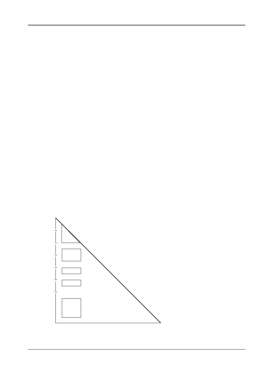
Let us see the following example with the graph and the shaft of elimination of [Figure 1.3-d] (nodes 8,9,
10 are not reproduced on the drawing).

SN4 (8,9,10)

SN3 (4,5,6,7)

SN2 (3)

SN1 (1,2)

Appear 1.3-d: Example of graph and shaft of elimination

Between brackets, one reads the numbers of the unknown factors of SN.
The elimination of the SN1 consists of:

1) assembly of columns 1 and 2 of the matrix initial, in a matrix of work, known as

frontal matrix before elimination. This matrix is of command 5, related to the unknown factors (1, 2, 4, 5,
6). (Because 1 and 2 is related to (4, 5, 6) only),

2) the elimination of the SN1 (of columns 1 and 2, according to the formulas [éq 1.1-7] and [éq 1.1-8] seen

previously),

3) arrangement of two columns 1 and 2 of the matrix, in a table Factor, which contains

columns of the total factorized matrix,

4) arrangement of the frontal matrix 1 of command 3 related to the unknown factors (4, 5, 6).

One makes the same thing with the SN2.
These two eliminations are illustrated by the figure [Figure 1.3-e], where one sees in grayed with hatching them
two frontal matrices.

frontal matrix 1

frontal matrix 2

table Factor

Appear 1.3-e

Code_Aster

Version

5.0

Titrate:

Method multifrontale

Date:

26/02/01

Author (S):

C. ROSE

Key:

R6.02.02-B

Page:

12/18

Manual of Reference

R6.06 booklet: Direct methods

HI-75/01/001/A

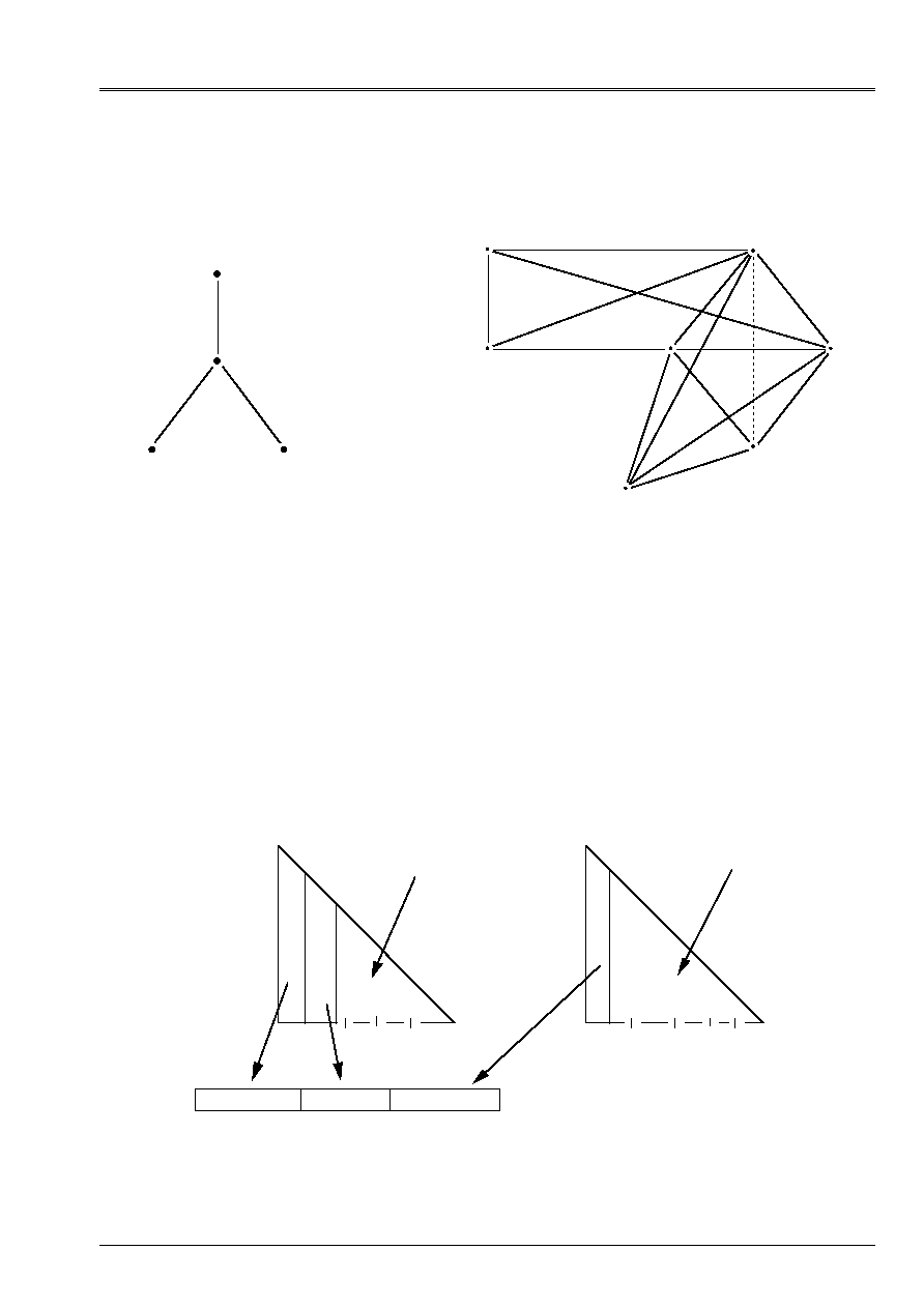
The elimination of the SN3 consists of:

the addition of the columns (4, 5, 6, 7) of the initial matrix, with the matrix of work of command 7, related to
unknown factors (4, 5, 6, 7, 8, 9, 10),

assembly of the frontal matrices 1 and 2 in this matrix of work,

the elimination of the columns (4, 5, 6, 7),

obtaining in additional Factor of four columns,

obtaining the frontal matrix 3d' command 3 (columns 8, 9, 10).

It is noticed that the frontal matrix 3 can line up in the place of the frontal matrices 1 and 2.
arrangement of these matrices requires a structure of pile where one piles up at the end of an elimination, and
where one depilates during the assembly. It is the maximum length of this pile which is minimized at the time of
the phase of sequence of execution.

The figure [Figure 1.3-f] illustrates the elimination of the SN3.

frontal matrix 1

stamp

frontal 2

frontal matrix 3

initial columns

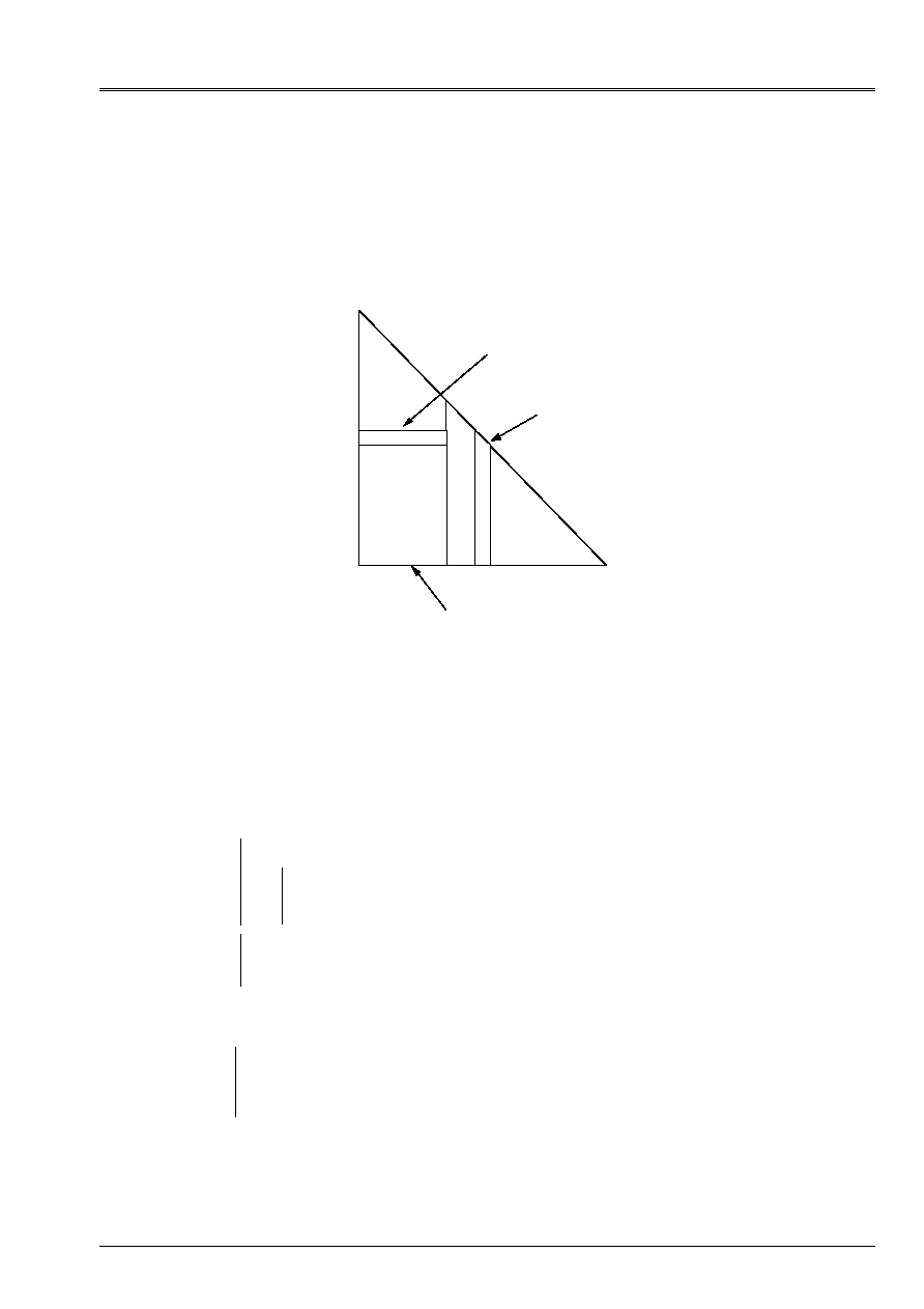
Appear 1.3-f: Elimination of the SN3

It is noticed that the coefficient

(white square on the figure [Figure 1.3-f]), comes from elimination

SN3, and that the initial term

With

is null (link in dotted on the figure [Figure 1.3-d].

One saw in paragraph 1.1 that the elimination of a column consisted of an operation of the type “saxpy”,
addition with a vector of the product of a vector by a scalar.
It is seen easily that the elimination of a super-node, groups columns, consists of an operation
of type “matrix-vector produces”. These operations consume the greatest part in calculating times,
work of factorization of the matrix. They are carried out by subroutines of
library BLAS, provided after being optimized on the majority of the computers. One sees on

appear [Figure 1.3-g] the column

update by the product of the matrix

[

]

With J

: :

and of

vector

[

]

With J

Code_Aster

Version

5.0

Titrate:

Method multifrontale

Date:

26/02/01

Author (S):

C. ROSE

Key:

R6.02.02-B

Page:

13/18

Manual of Reference

R6.06 booklet: Direct methods

HI-75/01/001/A

Factorization being finished, one has the matrix factorized in the shape of a table
compacted nonnull terms only. It is a storage of the type “Morse”. The table of index
total evoked in factorization symbolic system indicates, for each column of

, numbers of

line of each stored coefficient.

To J, 1: m

[

]

With J

1: N, J

[

]

With J

1: N, 1: m

[

]

Appear 1.3-g: Update of the column J by a product stamps * vector

1.4

Descent - Increase

Columns of

being stored in a compacted way, the descent is of type “saxpy” and

increase of the type produces scalar, these two operations being both indexed. I.e.
the algorithm of descent is coarsely the following, (while having initialized beforehand

second member of the system):

()

(

)

()

(

)

()

(saxpy indexed)

for

with

to make

for

to make

for

with

to make

total K

column

The increase, it, is written in the form:

()

(

)

N 1

indexed scalar product

for

varying

to make

total K

K column I

of with

Code_Aster

Version

5.0

Titrate:

Method multifrontale

Date:

26/02/01

Author (S):

C. ROSE

Key:

R6.02.02-B

Page:

14/18

Manual of Reference

R6.06 booklet: Direct methods

HI-75/01/001/A

Establishment and use in Code_Aster

The use of the multi-frontal method is accessible by the operator

NUME_DDL,

way

following:

naked =

NUME_DDL (matr_rigi: matr, storage: “MORSE”, or renum: “MDA”

renum: “MANDELEVIUM”); or renum: “MONGREL”

Two other methods of renumerotation are available: Approximate Degré minimum (MDA), which is
an alternative of the method of the degree minimum, and a method of encased dissection (MONGREL). They
are briefly described in appendices 1 and 2. It is enough to replace the value of renum by MDA, or
MONGREL.

This method is also available in

MECA_STATIQUE

STAT_NON_LINE

DYNA_NON_LINE

THER_LINEAIRE

THER_NON_LINE

with same logic.

Then, the operator will be used

FACT_LDLT

, the call being the same one as in the case of a matrix

stored according to the profile mode.

NUME_DDL

, it is indicated that the matrix to be factorized is arranged according to the mode

“MORSE”

and that

one asks for one of the two renumérotations of the “minimum dismantles”, or a renumerotation by
encased dissection (MONGREL).

In this case,

NUME_DDL

carry out the first three phases seen previously:

1) renumerotation,
2) factorization

symbolic system,

3) sequence

of execution.

These operations take into account the presence of “double-lagrange” and respect the command of D.D.L.
implied by the boundary conditions.

Moreover,

NUME_DDL

prepare cutting per blocks of the factorized matrix. Indeed, one saw that with

each elimination, one arranged in a table the columns of the factorized matrix. These columns
will be useful that at the time of the gone up descent/. They are never used for calculation of other columns. There is not
thus no interest to have them all in memory. They are arranged, in Code_Aster, under
form of a collection of objects JEVEUX length variable. These objects, blocks of columns, must
nevertheless to satisfy the following stress: each block corresponds to an integer of
“supernoeuds”. One cannot thus have the columns of same “a supernoeud” on several blocks.

Since one does not know the place in memory available during numerical factorization,
one decides in

NUME_DDL

that the maximum length of each block will be the max. one (on all SN)

sum lengths of the columns of SN.

(

)

(

)

Max

length neck

SNi

K SNi

max

, in summary

Code_Aster

Version

5.0

Titrate:

Method multifrontale

Date:

26/02/01

Author (S):

C. ROSE

Key:

R6.02.02-B

Page:

15/18

Manual of Reference

R6.06 booklet: Direct methods

HI-75/01/001/A

The operator

FACT_LDLT

use the pointers created by

NUME_DDL

and the initial matrix '

MORSE'

. It

create the matrix factorized in the shape of a collection of objects JEVEUX, as one saw
previously. A structure of data provisional is also necessary. It relates to the matrices
frontal. Two cases arise:

the pile of the frontal matrices can hold very whole in memory (in a table

monodimensional), in this case, one allocates an object JEVEUX and the algorithm multifrontal manages
then itself this space, by arranging the frontal matrix “mother” in the place of the matrices
“girls”,

it does not hold and, in this case, it is created in the shape of a collection of objects

JEVEUX, each frontal matrix being an object. For the elimination of the “supernoeud”

, it is necessary

at the same time in memory:

the block of factorized to which belongs it

SNi

the object stamps frontal

, like all the frontal matrices “girl” of

, which

will be destroyed after their use.

The frontal matrix

, it, will be stored until its use and its destruction. One

could, as it was made before, to release within the meaning of JEVEUX each frontal matrix after its
creation. That can involve then, in the event of weak memory available, a storage on disc
crippling in volume. Indeed, a destruction of object JEVEUX does not involve the destruction of sound
image on disc, and summons it lengths of the frontal matrices is enormous.

In short, it is necessary to be able to arrange simultaneously in memory:

a block of factorized,

the pile of the frontal matrices, in only one object if that holds, several objects if not.

One thus needs “sufficient” memory to use the method multifrontale. Second manner of
to arrange the pile allows the execution when the memory is sufficient, but émiettée.

When the memory is insufficient, it is necessary to start again the execution of

fact_ldlt

with a memory more

large.

Note:

In order to provide an order of magnitude, the large case-tests treated by Code_Aster, required
up to 20 or 25 megawords of memory for the pile of the frontal matrices. In the majority of
case the fact_ldlt resolution is used after many other operators, and does not profit any more
that of a émiéttée memory, or little of memory, (in particular during the use of
the operator

MODE_ITER_SIMULT

MODE_ITER_INV

, which allocates much place to the vectors

LANCZOS). The user wanting to carry out a very large case can have interest to proceed into two
stages, the second executant fact_ldlt in mode “continuation” and profiting then from a memory
not émiettée power station.

Code_Aster

Version

5.0

Titrate:

Method multifrontale

Date:

26/02/01

Author (S):

C. ROSE

Key:

R6.02.02-B

Page:

16/18

Manual of Reference

R6.06 booklet: Direct methods

HI-75/01/001/A

3 Bibliography

[1]

I. DUFF: Parallel implementation off multifrontal design ". Parallel computing 3, pp. 193-201
(1986)

[2]

C. ROSE: A method multifrontale for the direct resolution of the linear systems. Note
HI-76/93/008

[3]

Minimum year approximate dismantles ordering algorithm, Tim DAVIS, Patrick AMESTOY, Iain
DUFF, Technical Carryforward TR 94-039, (SIAM J. Matrix Analysis & Applications, flight 17, no.4,
(1996), pp. 886-905).

[4]

Minimum The evolution off the dismantles ordering ordering, A. George, J. Liu, SIAM review, flight 31
1989. One can also consult Internet sites following

: HTTP

://www.cerfacs.fr -

HTTP://ww.cise.ufl.edu/~davis

[5]

MONGREL: With software package for partitionning unstructured graphs, partitioning meshes, and
computing yarn oredering off sparse matrices Version 4.0. George Karypis &Vipin KUMAR

[6]

With fast and high quality MultiLevel Design for partitioning irregular graphs. SIAM newspaper one
Scientific Computing 1998, Flight 20 No 1. George Karypis & Vipin KUMAR

Code_Aster

Version

5.0

Titrate:

Method multifrontale

Date:

26/02/01

Author (S):

C. ROSE

Key:

R6.02.02-B

Page:

17/18

Manual of Reference

R6.06 booklet: Direct methods

HI-75/01/001/A

Appendix

Reference material of the method
“Approximate Minimum dismantles”

The algorithm of the “minimum dismantles” consists has to number the nodes of a graph in the ascending order of
numbers of their neighbor. Here is a simplified but essential description.

1) one forms the initial graph associated with the matrix digs to factorize,
2) one calculates the number of the neighbors of the nodes (their degree),
3) one numbers in first (then eliminates from the graph), the node having less neighbors (minimum degree),
4) one updates the graph of stage 1,
5) one turns over at stage 2.

The calculation of the degree of the nodes is an expensive operation in calculating times. The method “Approximate
Minimum dismantles “[bib3] proposes to reduce this cost. For that, instead of calculating the real degree of a node
one is satisfied with one raising (often equal, according to the authors, with the true degree), of easier calculation. Indeed with

run of elimination the true degree of the node

is equal to

, cardinal of the following unit:

{}

With

, where

the union is made on the whole of the neighbors

, previously eliminated, of

(terms of filling), and where

With

is the whole of the initial neighbors. In the approximate method

is replaced by

card (

With

) +

card

{}

, i.e. one neglects the intersection of

This method is described in [bib3] and the various alternatives of the algorithm of the “minimum dismantles” are
exposed in [bib4].

Appendix 2 Reference material Mongrel

The implementation of the module of renumerotation for matrices dig MONGREL is described in the note [bib5],
provided in the index mongrel-4.0/Doc. of the software. The algorithm used is described in [bib6]
It is also possible to consult following address Internet: HTTP://www.cs.umn.edu/~karypis

Mongrel is mainly a cutting tool of graphs (mesh), aiming at the 2 following goals:

to cut out a graph given out of p subgraphs having the closest possible sizes,

to minimize the size of the borders between the subgraphs.
The first goal aims at a good balance of parallelization on p processors and the second aims at minimizing
communications.

MONGREL uses an algorithm of partition of graphs on several levels, proceeding in the following way: with
each level one seeks separators (together of with dimensions), minimal sizes cutting the graph in
equal parts. MONGREL applies this principle to the renumerotation of the nodes of a graph while seeking to each
stage a separator dividing the graph into 2 subgraphs. The nodes of the first at the head are numbered
subgraph, then those of the second, then those of the separator. One applies then the same algorithm to the 2
under graphs in a recursive way.