
Code_Aster
®
Version
5.0
Titrate:
SDLD104 - Extrapolation of local measurements on a complete model
Date:
04/03/02
Author (S):
S. AUDEBERT, P. HERMANN
Key
:
V2.01.104-A
Page:
1/12
Manual of Validation
V2.01 booklet: Linear dynamics of the discrete systems
HT-62/01/012/A
Organization (S):
EDF/RNE/AMV, CS IF
Manual of Validation
V2.01 booklet: Linear dynamics of the discrete systems
V2.01.104 document
SDLD104 - Extrapolation of local measurements
on a complete model (discrete)
Summary:
It is about a test of linear dynamics discrete.
The goal is to test control PROJ_MESU_MODAL in the case of a discrete system. This control
allows to project experimental dynamic transitory answers in a certain number of points on
a modal base of a numerical modeling.
This test contains 2 modelings:
·
projection is done on a basic concept modal of type [mode_meca],
·
projection is done on a basic concept modal of type [base_modale].
For 2 modelings, the provided experimental measurements are identical and make it possible to test
seek nodes in opposite, the taking into account of a local orientation and the processing of one
sampling in constant time or not, for measurements in displacement.
In both cases, the reference solution is analytically given (by Maple); projection is
realized in the favorable configuration where the number of modes is equal to the number of measurements.
The answers in displacement obtained after projection are identical to displacements of reference
provided in data.
The values speeds and the accelerations deduced from the displacements obtained after projection are
close relations of those obtained analytically. The weak noted variations are due to the errors of approximation
generated by the determination via a linear diagram in time of speeds and accelerations.

Code_Aster
®
Version
5.0
Titrate:
SDLD104 - Extrapolation of local measurements on a complete model
Date:
04/03/02
Author (S):
S. AUDEBERT, P. HERMANN
Key
:
V2.01.104-A
Page:
2/12
Manual of Validation
V2.01 booklet: Linear dynamics of the discrete systems
HT-62/01/012/A
1
Problem of reference
1.1
Description of the system
We consider the system represented by the diagram below:
1.2
Masses and rigidity
The three springs are of identical rigidity:
K
= 1000 NR/Mr.
The two masses are equal to
m
= 10 kg.
1.3
Boundary conditions and loading
The two ends are embedded.
The loading is a thrust load in traction applied to the mass
m
1
, sinusoidal according to
time, of pulsation
.
X
1
X
2
m
m
K
K
K

Code_Aster
®
Version
5.0
Titrate:
SDLD104 - Extrapolation of local measurements on a complete model
Date:
04/03/02
Author (S):
S. AUDEBERT, P. HERMANN
Key
:
V2.01.104-A
Page:
3/12
Manual of Validation
V2.01 booklet: Linear dynamics of the discrete systems
HT-62/01/012/A
2
Reference solutions
2.1
Method of calculation used for the reference solution
The analytical solution of this problem is presented below.
·
Modes and frequencies of vibration:
The following system characterizes the dynamics of the masses:
MX
kx
kx
MX
kx
kx
&&
&&
1
1
2
2
2
1
2
0
2
0
+
-
=
+
-
=
éq 2.1-1
What is equivalent to the following system:
(
) (
)
(
)
(
)
m X
X
K X
X
m X
X
K X
X
& & &&
& & &&
1
2
1
2
1
2
1
2
0
3
0
+
+
+
=
-
+
-
=
éq 2.1-2
The 2 Eigen frequencies of the system are thus given by:
1
2
3
=
=
K
m
K
m
and
éq
2.1-3
and the associated modal deformations are:
1
2
1
1
1
1
=
= -
and
éq
2.1-4
The generalized matrices are:
M
M
K
K
=
=
-
-
=
=
=
-
-
-
-
=
T
T
m
m
m
m
K
K
K
K
K
K
1
1
1
1
0
0
1
1
1
1
2
0
0
2
1
1
1
1
2
2
1
1
1
1
2
0
0
6
éq
2.1-5
·
Transitory answer:
The sinusoidal effort is applied to the first mass:
()
F
= 10 sin
T

Code_Aster
®
Version
5.0
Titrate:
SDLD104 - Extrapolation of local measurements on a complete model
Date:
04/03/02
Author (S):
S. AUDEBERT, P. HERMANN
Key
:
V2.01.104-A
Page:
4/12
Manual of Validation
V2.01 booklet: Linear dynamics of the discrete systems
HT-62/01/012/A
The checked dynamic system is as follows:
MX KX F
& & +
=
éq 2.1-6
While projecting on the basis of clean mode, we obtain:
T
T
T
M
K
F
& & +
=
éq
2.1-7
That is to say:
()
2
0
0
2
2
0
0
6
1
1
1
1
1
0
1
2
1
2
m
m
K
K
T
+
=
-
&&
&&
sin
éq
2.1-8
We thus end to the following uncoupled system:
()
()
m
K
T
m
K
T
&&
sin
&&
sin
1
1
2
2
1
2
3
1
2
+
=
+
=
éq
2.1-9
The solution of this system is given by:
()
()
()
()
(
)
()
()
()
()
(
)
1
1
1
1
1
12
2
2
2
2
2
2
22
2
2
2
T
With
T
B
T
T
m
T
With
T
B
T
T
m
=
+
+
-
=
+
+
-
cos
sin
sin
cos
sin
sin
éq
2.1-10
Displacements in physical space are obtained by the formula of Ritz:
X
= = =
-
= +
X
X
1
2
1
2
1
2
1
2
1
1
1
1
éq
2.1-11
One deduces the expressions from them from:
()
()
X T
X T
1
2
and
éq
2.1-12
()
()
()
()
()
()
()
()
()
()
()
()
X T
With
T
B
T
With
T
B
T
T
m
X T
With
T
B
T
With
T
B
T
T
m
1
1
1
1
1
2
2
2
2
12
2
22
2
2
1
1
1
1
2
2
2
2
12
2
22
2
2
1
1
2
1
1
=
+
+
+
+
-
+
-
=
+
-
+
+
-
-
-
cos
sin
cos
sin
sin
cos
sin
cos
sin
sin

Code_Aster
®
Version
5.0
Titrate:
SDLD104 - Extrapolation of local measurements on a complete model
Date:
04/03/02
Author (S):
S. AUDEBERT, P. HERMANN
Key
:
V2.01.104-A
Page:
5/12
Manual of Validation
V2.01 booklet: Linear dynamics of the discrete systems
HT-62/01/012/A
At the initial moment, the system is at rest, from where final expressions of
()
X T
1
and
()
X T
2
:
()
()
()
()
()
()
()
()
()
()
X T
m
T
T
T
T
X T
m
T
T
T
T
1
1
1
12
2
2
2
22
2
2
1
1
12
2
2
2
22
2
1
2
1
2
=
-
-
+
-
-
=
-
-
-
-
-
sin
sin
sin
sin
sin
sin
sin
sin
éq
2.1-13
Speeds of the two masses are calculated by deriving displacements compared to time:
()
()
()
()
()
()
()
()
()
()
&
cos
cos
cos
cos
&
cos
cos
cos
cos
X T
m
T
T
T
T
X T
m
T
T
T
T
1
1
12
2
2
22
2
2
1
12
2
2
22
2
2
2
=
-
-
+
-
-
=
-
-
-
-
-
éq
2.1-14
Accelerations of the two masses are calculated by deriving speeds compared to time:
()
()
()
()
()
()
()
()
()
()
&&
sin
sin
sin
sin
&&
sin
sin
sin
sin
X T
m
T
T
T
T
X T
m
T
T
T
T
1
1
1
12
2
2
2
22
2
2
1
1
12
2
2
2
22
2
2
2
=
-
-
+
-
-
=
-
-
-
-
-
éq 2.1-15
2.2
Results of reference
The comparison of the results relates to displacements, speeds and accelerations along the axis of
two masses, at five different moments.
2.3
Uncertainty on the solution
The reference solution is exact.
The discrete model represents perfectly the problem arising (the modal base is complete; there is not
thus not of approximation related to a possible modal truncation). The number of modes of the base
of modal projection is equal to the number of measurements, therefore the solution of the inversion is exact (by
opposition to an approximate solution of a generalized opposite problem). If the search of the nodes in
opposite is good, the displacements obtained after projection must be in perfect adequacy
with the experimental values. Speeds and accelerations are determined by derivation of
modal contributions identified via a diagram of linear approximation in time, thus being able
to generate some errors.
Code_Aster
®
Version
5.0
Titrate:
SDLD104 - Extrapolation of local measurements on a complete model
Date:
04/03/02
Author (S):
S. AUDEBERT, P. HERMANN
Key
:
V2.01.104-A
Page:
6/12
Manual of Validation
V2.01 booklet: Linear dynamics of the discrete systems
HT-62/01/012/A
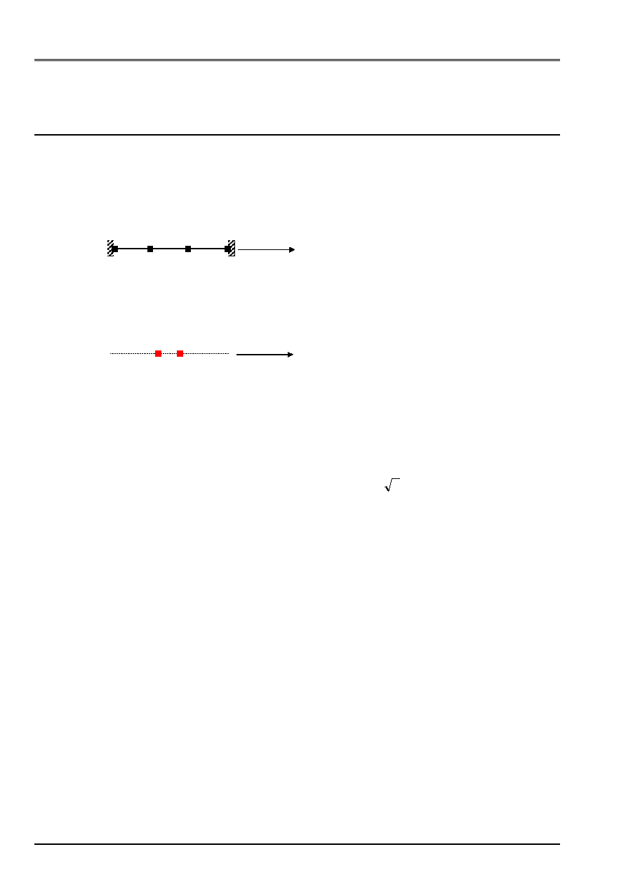
3 Modeling
With
3.1
Characteristics of modeling and the mesh
·
Numerical mesh:
The numerical mesh is carried out directly with the format ASTER. It comprises 4 nodes and 3
discrete meshs.
·
Experimental mesh:
The mesh of measurement includes/understands only 2 specific elements and 2 nodes:
3.2
Characteristics of the measurements
The provided experimental measurements are:
·
With the N3 node:
The data are the axial displacements, multiplied by (
2
/2), and applied in the direction
X. the local orientation indicated in the command file is (45. 0. 0.)
The sampling of time is constant: initial time is 0 S, the pitch of time is 10
3
S and it
a many moments are 1001 (i.e until a final time of 1 S).
·
With the node N2:
The data are the axial displacements, applied in the direction
X
.
The sampling of time is variable: every moment is indicated of 0 S to 1 S, by pitch of
10
3
S (1001 moments on the whole).
The values result from the analytical calculation carried out with Maple.
3.3
Characteristics of the modal base
The two only modes are stored in a concept of the type [mode_meca] created by the control
MODE_ITER_SIMULT. Their Eigen frequencies are identical to the analytical Eigen frequencies.
m
m
K
K
K
X
N1
(x=0.)
N2
(x=0.1)
N4
(x=0.3)
N3
(x=0.2)
X
N3
(x=0.18)
N2
(x=0.12)

Code_Aster
®
Version
5.0
Titrate:
SDLD104 - Extrapolation of local measurements on a complete model
Date:
04/03/02
Author (S):
S. AUDEBERT, P. HERMANN
Key
:
V2.01.104-A
Page:
7/12
Manual of Validation
V2.01 booklet: Linear dynamics of the discrete systems
HT-62/01/012/A
3.4 Functionalities
tested
Controls
AFFE_CARA_ELEM
DISCRETE
ORIENTATION
IDENTIFY
CARA
“ANGL_NAUT”
“LOCAL”
'M_T_D_N
“K_T_D_L'
AFFE_CHAR_MECA
DDL_IMPO
ALL
NODE
AFFE_MODELE
ALL
“MECHANICAL” “DIST_T'
ASSE_MATRICE
CALC_MATR_ELEM OPTION
“MASS_MECA”
“RIGI_MECA”
MODE_ITER_SIMULT CALC_FREQ
OPTION
'
BANDE'
NUME_DDL
NUME_DDL_GENE
PROJ_MATR_BASE
PROJ_MESU_MODAL
MEASURE
REGULARIZATION
REST_BASE_PHYS TOUT_CHAM
“YES”
TEST_RESU NOM_CHAM
CRITERION
“DEPL”
“QUICKLY”
“ACCE”
“RELATIVE”

Code_Aster
®
Version
5.0
Titrate:
SDLD104 - Extrapolation of local measurements on a complete model
Date:
04/03/02
Author (S):
S. AUDEBERT, P. HERMANN
Key
:
V2.01.104-A
Page:
8/12
Manual of Validation
V2.01 booklet: Linear dynamics of the discrete systems
HT-62/01/012/A
4
Results of modeling A
4.1 Values
tested
Identification Reference
Code_Aster difference
with
T
= 0.1 S
1.745 10
4
1.745
10
4
0.01
%
with
T
= 0.3 S
6.797 10
4
6.797
10
4
0.01
%
DEPL_X
with the node N2
with
T
= 0.5 S
1.217 10
3
1.217
10
3
0.01
%
(m) (mass
1)
with
T
= 0.7 S
5.214 10
4
5.214
10
4
0.01
%
with
T
= 0.9 S
9.031 10
4
9.031
10
4
0.00
%
with
T
= 0.1 S
9.154 10
6
9.154
10
6
0.00
%
with
T
= 0.3 S
6.414 10
4
6.414
10
4
0.00
%
DEPL_X
with the N3 node
with
T
= 0.5 S
8.636 10
4
8.636
10
4
0.00
%
(m) (mass
2)
with
T
= 0.7 S
1.107 10
4
1.107
10
4
0.03
%
with
T
= 0.9 S
1.633 10
3
1.633
10
3
0.02
%
with
T
= 0.1 S
4.586 10
3
4.616
10
3
0.65
%
with
T
= 0.3 S
7.598 10
3
7.663
10
3
0.85
%
VITE_X
with the node N2
with
T
= 0.5 S
1.581 10
4
8.000
10
5
7.81
10
5
m/s
(m/s) (mass
1)
with
T
= 0.7 S
9.382 10
3
9.354
10
3
0.30
%
with
T
= 0.9 S
7.481 10
3
7.537
10
3
0.75
%
with
T
= 0.1 S
4.328 10
4
4.405
10
4
1.79
%
with
T
= 0.3 S
3.671 10
3
3.640
10
3
0.84
%
VITE_X
with the N3 node
with
T
= 0.5 S
1.539 10
2
1.536
10
2
0.20
%
(m/s) (mass
2)
with
T
= 0.7 S
2.453 10
2
2.457
10
2
0.15
%
with
T
= 0.9 S
1.899 10
2
1.912
10
2
0.68
%
with
T
= 0.1 S
6.112 10
2
6.100
10
2
0.20
%
with
T
= 0.3 S
1.306 10
1
1.300
10
1
0.46
%
ACCE_X
with the node N2
with
T
= 0.5 S
1.571 10
1
1.600
10
1
1.85
%
(m/s
2
) (mass
1) with
T
= 0.7 S
5.657 10
2
5.800
10
2
2.53
%
with
T
= 0.9 S
1.124 10
1
1.130
10
1
0.53
%
with
T
= 0.1 S
1.562 10
2
1.618
10
2
3.58
%
with
T
= 0.3 S
6.031 10
2
6.223
10
2
3.18
%
ACCE_X
with the N3 node
with
T
= 0.5 S
5.102 10
2
5.374
10
2
5.33
%
(m/s
2
) (mass
2) with
T
= 0.7 S
7.428 10
2
7.043
10
2
5.19
%
with
T
= 0.9 S
2.364 10
1
2.263
10
1
4.28
%
Note:
Speed with the node N2 at the moment T = 0.5 S being relatively close to zero, the comparison
is realized for this case in absolute value.
4.2 Parameters
of execution
Version: STA5 (5.05)
Machine: CLASTER
Overall dimension memory: 100 Mo
Time CPU To use: 9.05 seconds
Code_Aster
®
Version
5.0
Titrate:
SDLD104 - Extrapolation of local measurements on a complete model
Date:
04/03/02
Author (S):
S. AUDEBERT, P. HERMANN
Key
:
V2.01.104-A
Page:
9/12
Manual of Validation
V2.01 booklet: Linear dynamics of the discrete systems
HT-62/01/012/A
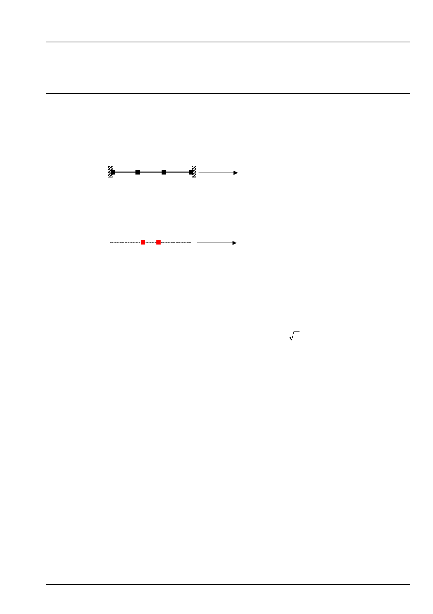
5 Modeling
B
5.1
Characteristics of modeling and the mesh
·
Numerical mesh:
The numerical mesh is carried out directly with the format ASTER. It comprises 4 nodes and 3
discrete meshs.
·
Experimental mesh:
The mesh of measurement includes/understands only 2 specific elements and 2 nodes:
5.2
Characteristic of the measurements
The provided experimental measurements are:
·
With the N3 node:
The data are the axial displacements, multiplied by (
2
/2), and applied in the direction
X
. The local orientation indicated in the command file is (45. 0. 0.)
The sampling of time is constant: initial time is 0 S, the pitch of time is 10
3
S and it
a many moments are 1001 (i.e until a final time of 1 S).
·
With the node N2:
The data are the axial displacements, applied in direction X.
The sampling of time is variable: every moment is indicated of 0 S to 1 S, by pitch of
10
3
S (1001 moments on the whole).
The values result from the analytical calculation carried out with Maple.
5.3
Characteristics of the modal base
The two only modes are stored in a concept of the type [base_modale], created by the control
DEFI_BASE_MODALE. The interface, of Craig-Bampton type, is placed on the degree of freedom in
following displacement
X
node N2 (corresponding to the mass
m
1). The modal base thus contains
a dynamic mode (with locked N2) and a static mode.
m
m
K
K
K
X
N1
(x=0.)
N2
(x=0.1)
N4
(x=0.3)
N3
(x=0.2)
X
N3
(x=0.18)
N2
(x=0.12)

Code_Aster
®
Version
5.0
Titrate:
SDLD104 - Extrapolation of local measurements on a complete model
Date:
04/03/02
Author (S):
S. AUDEBERT, P. HERMANN
Key
:
V2.01.104-A
Page:
10/12
Manual of Validation
V2.01 booklet: Linear dynamics of the discrete systems
HT-62/01/012/A
5.4 Functionalities
tested
Controls
AFFE_CARA_ELEM
DISCRETE
CARA
'M_T_D_N
“K_T_D_L'
ORIENTATION
“ANGL_NAUT”
IDENTIFY
“LOCAL”
AFFE_CHAR_MECA
DDL_IMPO
ALL
NODE
AFFE_MODELE
ALL
PHENOMENON
MODELING
“YES”
“MECHANICAL”
“DIST_T'
ASSE_MATRICE
CALC_MATR_ELEM OPTION
“MASS_MECA”
“RIGI_MECA”
CONVENTIONAL DEFI_BASE_MODALE
DEFI_INTERF_DYNA INTERFACES
MODE_ITER_SIMULT CALC_FREQ
OPTION
'
BANDE'
NUME_DDL
NUME_DDL_GENE
PROJ_MATR_BASE
PROJ_MESU_MODAL
MEASURE
REGULARIZATION
REST_BASE_PHYS TOUT_CHAM
“YES”
TEST_RESU NOM_CHAM
CRITERION
“DEPL”
“QUICKLY”
“ACCE”
“RELATIVE”

Code_Aster
®
Version
5.0
Titrate:
SDLD104 - Extrapolation of local measurements on a complete model
Date:
04/03/02
Author (S):
S. AUDEBERT, P. HERMANN
Key
:
V2.01.104-A
Page:
11/12
Manual of Validation
V2.01 booklet: Linear dynamics of the discrete systems
HT-62/01/012/A
6
Results of modeling B
6.1 Values
tested
Identification Reference
Code_Aster difference
with
T
= 0.1 S
1.745 10
4
1.745
10
4
0.01
%
with
T
= 0.3 S
6.797 10
4
6.797
10
4
0.01
%
DEPL_X
with the node N2
with
T
= 0.5 S
1.217 10
3
1.217
10
3
0.01
%
(m) (mass
1)
with
T
= 0.7 S
5.214 10
4
5.214
10
4
0.01
%
with
T
= 0.9 S
9.031 10
4
9.031
10
4
0.00
%
with
T
= 0.1 S
9.154 10
6
9.154
10
6
0.00
%
with
T
= 0.3 S
6.414 10
4
6.414
10
4
0.00
%
DEPL_X
with the N3 node
with
T
= 0.5 S
8.636 10
4
8.636
10
4
0.00
%
(m) (mass
2)
with
T
= 0.7 S
1.107 10
4
1.107
10
4
0.03
%
with
T
= 0.9 S
1.633 10
3
1.633
10
3
0.02
%
with
T
= 0.1 S
4.586 10
3
4.616
10
3
0.65
%
with
T
= 0.3 S
7.598 10
3
7.663
10
3
0.85
%
VITE_X
with the node N2
with
T
= 0.5 S
1.581 10
4
8.000
10
5
7.81
10
5
m/s
(m/s) (mass
1)
with
T
= 0.7 S
9.382 10
3
9.354
10
3
0.30
%
with
T
= 0.9 S
7.481 10
3
7.537
10
3
0.75
%
with
T
= 0.1 S
4.328 10
4
4.405
10
4
1.79
%
with
T
= 0.3 S
3.671 10
3
3.640
10
3
0.84
%
VITE_X
with the N3 node
with
T
= 0.5 S
1.539 10
2
1.536
10
2
0.20
%
(m/s) (mass
2)
with
T
= 0.7 S
2.453 10
2
2.457
10
2
0.15
%
with
T
= 0.9 S
1.899 10
2
1.912
10
2
0.68
%
with
T
= 0.1 S
6.112 10
2
6.100
10
2
0.20
%
with
T
= 0.3 S
1.306 10
1
1.300
10
1
0.46
%
ACCE_X
with the node N2
with
T
= 0.5 S
1.571 10
1
1.600
10
1
1.85
%
(m/s
2
) (mass
1) with
T
= 0.7 S
5.657 10
2
5.800
10
2
2.53
%
with
T
= 0.9 S
1.124 10
1
1.130
10
1
0.53
%
with
T
= 0.1 S
1.562 10
2
1.618
10
2
3.58
%
with
T
= 0.3 S
6.031 10
2
6.223
10
2
3.18
%
ACCE_X
with the N3 node
with
T
= 0.5 S
5.102 10
2
5.374
10
2
5.33
%
(m/s
2
) (mass
2) with
T
= 0.7 S
7.428 10
2
7.043
10
2
5.19
%
with
T
= 0.9 S
2.364 10
1
2.263
10
1
4.28
%
Note:
Speed with the node N2 at the moment T = 0.5 S being relatively close to zero, the comparison
is realized for this case in absolute value.
6.2 Parameters
of execution
Version: STA5 (5.05)
Machine: CLASTER
Overall dimension memory: 100 Mo
Time CPU To use: 9.24 seconds

Code_Aster
®
Version
5.0
Titrate:
SDLD104 - Extrapolation of local measurements on a complete model
Date:
04/03/02
Author (S):
S. AUDEBERT, P. HERMANN
Key
:
V2.01.104-A
Page:
12/12
Manual of Validation
V2.01 booklet: Linear dynamics of the discrete systems
HT-62/01/012/A
7
Summary of the results
For two modelings, the answers in displacement obtained after projection are identical
with the displacements of reference calculated analytically with Maple and provided in data.
Values speeds and the accelerations deduced from the displacements obtained after projection
are close to those obtained analytically. The weak noted variations are due to the errors
of approximation generated by the determination by a linear diagram in time speeds and
accelerations.