Derivation of the theorem for one-dimensional flow

Consider a stream tube in an one-dimensional flow as sketched. we remind ourselves that the flow takes place entirely through the stream tube and there is no flow across it, i.e., in a direction normal to it. Let is consider a system S in the flow. Let us prescribe a control volume CV coincident with it at time t₀ (Fig.3.18). We recall that the system is an entity of fixed mass and is allowed to move and deform. On the other hand a control volume has fixed a boundary, which we denote as CS. In this analysis we keep it stationary. After the lapse of time $\Delta t$ i.e., at time $t_0+\Delta$ we find that the control volume remains at the same position, I+II while the system has moved to occupy the position II + III. We see that during the time interval mass contained in region I has entered the control volume and that in III has left the control volume.

Figure 3.18: Control Volume and system for an one-dimensional flow

 

 

Consider an extensive property N associated with the control volume. By definition we have,

$$\left. {dN_s} \over {dt} \right)~=~\lim_{\Delta t \rightarrow 0} {{N_s(t_0+\Delta t) - N_s(t_0)} \over {\Delta t}}$$ (3.16)

where subscript denotes a system.

Further we have at $t_0+\Delta t$

$$N_s(t_0+\Delta t)~ =~(N_{II}+N_{III})~ \texttt{at}~(t_0+\Delta t)$$

$$= (N_{CV}~-~N_I~+~N_{III}) ~\texttt{at}~ (t_0+\Delta t)$$ (3.17)

On substituting these into Eq.3.16 and noting that at t₀ the system and the control volume coincide, i.e., $N_s(t_0) = N_{CV}(t_0)$, we have

$$\left. {{dN} \over {dt}} \right)_s~=~{\lim_{\Delta t \rightarrow... ...III} \right](t_0+\Delta t)~~-~~\left[ N_{CV} \right](t_0)} \over {\Delta t}}}$$ (3.18)

By readjusting the terms we have,

$$\left. {{dN} \over {dt}} \right)_s~ =~{\lim_{\Delta t \rightarrow 0} {{ \left[ N_{CV}(t_0+\Delta t) - N_{CV}(t_0) \right]} \over {\Delta t}}}$$

$$+ \lim_{\Delta t \rightarrow 0} {{N_{III}(t_0~+~\Delta t)} \over {\Delta t} }$$

$$- \lim_{\Delta t \rightarrow 0} {{N_{I}(t_0~+~\Delta t)} \over {\Delta t} }$$ (3.19)

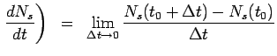
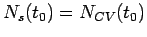
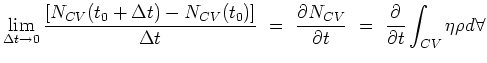
We can now take up each of the three limits on the RHS of the above equation.

The first limit gives,

$$\lim_{\Delta t \rightarrow 0} {{{{ \left[ N_{CV}(t_0+\Delta t) -... ...\over \partial t}~=~{\partial \over \partial t} \int_{CV} \eta \rho d \forall$$ (3.20)

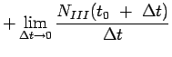
recalling that N is an extensive property and $\eta$ is the corresponding intensive property such that $N=\eta m$ where m is the mass given by $\rho$ times volume, i.e, $\rho \times d \forall$.

The second limit, which gives the rate of change of N within III could be written as

$$\lim_{\Delta t \rightarrow 0} {{N_{III}(t_0~+~\Delta t)} \over {... ...htarrow 0} \left[ {\eta \rho \forall} \over {\Delta t} \right](t_0~+~\Delta t)$$ (3.21)

The right hand side simply the rate at which N is going out of the control volume though the boundary, i.e., the control surface at right and is equal to

$$\left[ \eta \rho A V \right]_{out}$$ (3.22)

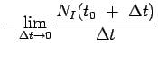
where A is the area of cross section of III, V is the velocity normal to the area.

Similarly we have for I, i.e., the rate at which N enters the control volume through the boundary or control surface at left,

$$\left[ \eta \rho A V \right]_{in}$$ (3.23)

Upon substituting Eqns. 3.20,3.22 and 3.23 into Eqn. 3.19, we have

$$\left. {{dN} \over {dt}} \right)_s~=~~{\partial \over \partial t}... ...~~+~~ \left[ \eta \rho A V \right]_{out}~~-~~ \left[ \eta \rho A V \right]_{in}$$ (3.24)

Eqn. 3.24 is the Reynolds Transport equation for the control volume considered. Each of the terms in the equation tells something significant. Putting the equation is words we have,

Rate of change of property N within the system =

Rate of change of property N within the control volume + Rate of outflow of property N through the control surface - Rate of inflow of property through the control surface.

which seems very obvious.

The above result can be generalised to any control volume of any shape, but fixed in space. Let us now consider such a general control volume as shown in Fig.3.19 . For such a control volume it is difficult to define an inlet boundary and an outlet boundary. It is best to consider the net flow of property N into the control volume. Accordingly, the above verbal equation is written as

Rate of change of property N within the system =

Rate of change of property N within the control volume + Net rate of change of property N through the control surface

Figure3.19: General Control Volume and System

 

Whether the flow at any small segment of control surface is an inflow or an outflow is decided by the direction of the velocity vector and that of the area vector at that segment. Consider a small area $\overrightarrow{d}A$ at the control surface (Fig.3.19 ). Let the velocity acting upon it be $\overrightarrow{V}$. The rate at which property N escapes or enters the control volume through $d\overrightarrow{A}$ depends upon the velocity component normal to $d\overrightarrow{A}$, i.e, $\overrightarrow{V}.d\overrightarrow{A}$. In fact the rate of flow of N through $d\overrightarrow{A}$ is given by

$$\eta \rho \overrightarrow{V}.d\overrightarrow{A}$$ (3.25)

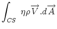
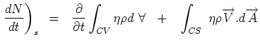
Integrating this for the entire control surface gives the net rate of flow of N into the control volume. I.e,

$$\int_{CS}~\eta \rho \overrightarrow{V}.d\overrightarrow{A}$$ (3.26)

Consequently we can write the Reynolds Transport theorem for a general control volume as

$$\left. {{dN} \over {dt}} \right)_s~=~~{\partial \over \partial t}... ...ho d ~ \forall~~+~~ \int_{CS}~\eta \rho \overrightarrow{V}.d\overrightarrow{A}$$ (3.27)

Abstract as it seems, Eqn. 3.27 simplifies when we consider concrete control volumes and many times becomes self-evident. This will become clear as we consider many applications of the Reynolds Transport theorem.

(c) Aerospace, Mechanical & Mechatronic Engg. 2005
University of Sydney