Flow through a Sharp-edged Orifice

Consider an orifice plate placed in a pipe flow as shown in Fig.3.25 . We assume that the thickness of the plate is small in comparison to the pipe diameter. Let the orifice be sharp edged. The effect of a rounded plate is a matter of detail and will not be considered here.

Figure 3.25: Flow through an Orifice Body

 

A fully developed flow prevails at the upstream of the orifice. The presence of the orifice makes the flow accelerate through it thus increasing the velocity. It may appear that the flow fills the orifice completely and expands downstream of it. But this is not true. As the flow expands downstream it cannot fill the entire diameter of the pipe at once. It requires a distance before it does. A recirculating flow develops immediate downstream of the nozzle. As a consequence the smallest diameter of flow is not equal to the orifice diameter, but smaller than it. The position of the smallest diameter occurs downstream of the orifice.

We can deduce the flow rate through the pipe by measuring the pressure difference upstream of the nozzle and at the orifice.

We make a few assumptions about the flow as follows -

1. The flow is steady
2. The flow is incompressible
3. There is no friction or losses
4. The velocities at sections (1) and (2) are uniform, i.e, they do not vary in a radial direction.
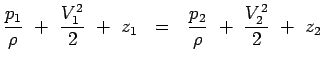
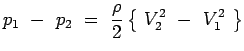
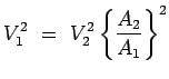
5. The pipe is horizontal, i.e., z is the same at (1) and (2), i.e., z₁ = z₂. This assumption can be relaxed easily. It is possible to have a fluid flowing through an inclined pipe. Then the gz term does not cancel out from LHS and RHS of the Bernoulli Equation.

The equations we consider are (a) Continuity and (b) Bernoulli equations.

a) Continuity Equation.

$$\rho_1~A_1~V_1~=~\rho_2~A_2~V_2$$ (3.78)

b) Bernoulli Equation

$${p_1 \over \rho}~+~{V_1^2 \over 2}~+~{z_1}~~=~~{p_2 \over \rho}~+~{V_2^2 \over 2}~+~z_2$$ (3.79)

The Bernoulli Equation gives,

$$p_1~-~p_2~=~{\rho \over 2} \left\{~ V_2^2~-~V_1^2~\right \}$$ (3.80)

Noting from Continuity  Equation that

$$V_1^2~=~V_2^2 \left\{ A_2 \over A_1 \right\}^2$$

$$p_1~-~p_2~=~{{\rho~V_2^2} \over 2} \left\{ 1~-~\left( A_2 \over A_1 \right)^2~\right \}$$ (3.81)

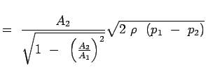
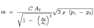
Solving for V₂ we have,

$$V_2~=~\sqrt{{2~(p_1~-~p_2)} \over {\rho~ \left[ 1~-~\left(A_2 \over A_1 \right)^2 \right]}}$$ (3.82)

Consequently, the mass flow rate becomes,

$$\dot{m}~ =\rho~A_2~\sqrt{{2~(p_1~-~p_2)} \over {\rho~ \left[ 1~-~\left(A_2 \over A_1 \right)^2 \right]}}$$

$$=~{{A_2} \over \sqrt{{ 1~-~\left(A_2 \over A_1 \right)^2 }}}{\sqrt{2~\rho~{~(p_1~-~p_2)}}}$$ (3.83)

The above equation gives the mass flow rate through the pipe in terms of the pressure drop and the areas. The equation gives only a theoretical value. In order to obtain a more realistic value one need to substitute the actual area at the minimum cross section or the Vena Contracta. This is not easy to measure. In addition losses may not be negligible as we have assumed. Extent of losses is a function of the Reynolds number. In practice, a Coefficient of Discharge is defined such that

$$\dot{m}~= ~{{C~A_2} \over \sqrt{{1~-~\left(A_2 \over A_1 \right)^2 }}}{\sqrt{2~\rho~{~(p_1~-~p_2)}}}$$ (3.84)

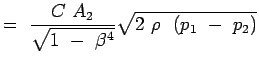
Further if we define a ratio of diameters $\beta$ such that

$$\beta = {D_2 \over D_1 }$$

$$\dot{m}~ = ~{{C~A_2} \over \sqrt{{1~-~\beta^4 }}}{\sqrt{2~\rho~{~(p_1~-~p_2)}}}$$ (3.85)

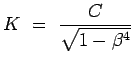
Sometimes the ratio $1 / \sqrt{1-\beta^4}$ is referred to as Velocity of Approach Factor. Again it is usual to combine this and the Discharge Coefficient to define a Flow Coefficient given by

$$K~=~{C \over \sqrt{1-\beta^4}}$$ (3.86)

Consequently the mass flow rate is given by,

$$\dot{m}~= ~K~A_2 \sqrt{2~\rho~~(p_1~-~p_2)}$$ (3.87)

Thus the mass flow rate for a pipe can be calculated with the knowledge of pressure drop, the orifice diameter and the coefficient K. Extensive data exists in handbooks on the coefficient K.

Pressure drop is usually measured by using a manometer as shown in Fig. 3.25. Now the pressure drop is obtained as h, the height of a liquid column (which may be mercury). Accordingly the alternate form of Eqn.3.87 is

$$\dot{m}~= ~K~A_2 \sqrt{2~\rho~g~h}$$ (3.88)

(c) Aerospace, Mechanical & Mechatronic Engg. 2005
University of Sydney