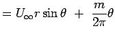
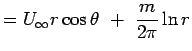
Uniform Flow and a Source

Let us now place a source in the path of a uniform flow. The stream function and the velocity potential for the resulting flow are given by adding the two stream functions and velocity potentials as follows,

$$\psi = \psi_{UF} + \psi_{S}$$

$$=U_\infty r\sin \theta + {m \over {2\pi}} \theta$$ (4.89)

$$\phi = \phi_{UF} + \phi_{S}$$

$$=U_\infty r\cos \theta + {m \over {2\pi}} \ln r$$ (4.90)

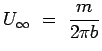
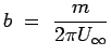
One of the interesting features to determine for the resulting force is the stagnation point of the flow, i.e., where the velocity goes to zero.

One could calculate this from the equations. It is clear that for this flow the stagnation point will occur on the x-axis. The location can be arrived at purely intuitionally. The source produces a radial flow of magnitude

$$v_r = {m \over {2r}}$$

while the uniform flow produces a velocity of U in the positive x-direction. When these two cancel out at a point we have the stagnation point. A negative radial flow that can cancel the uniform flow is possible only to the left of the x-axis, say at x = -b. Hence,

$$U_\infty = {m \over {2 \pi b}}$$

$$b = {m \over {2 \pi U_\infty}}$$ (4.91)

At x = -b, we have $\theta=\pi$ and r = b. Substituting these values in the expression for $\psi$, i.e., Eqn. 4.89 we get the value of $\psi$ at the stagnation point to be

$$\psi_{stagn} = {m \over 2}$$ (4.92)

An equation to the streamline passing through the stagnation point, i.e., stagnation streamline is obtained as follows,

$${m \over 2} = U_\infty r \sin \theta + {b U_\infty \theta}$$

$$U_\infty \pi b = U_\infty r \sin \theta + {b U_\infty \theta}$$

$$r = {{b(\pi - \theta)} \over {\sin \theta}}  or  y = {{b(\pi - \theta)}}$$ (4.93)

Figure 4.24: Flow about Rankine Half Body

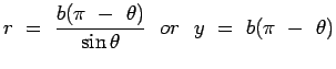
The streamlines for this flow are sketched in Fig.4.24. It is clear that we can make the stagnation streamline the solid body. In fact any streamline of a flow can be treated as a solid body since there is no flow across it. In the present example if we ignore the streamlines inside the "body" we have described the flow about a solid body given by Eqn. 4.25. This body is referred to as a Rankine Half Body as it is "open" at the right hand end.

Limits of $\theta$ for this body are 0 and $2 \pi$. At these values we have y approaching $\pm \pi b$, which is called the Half Width of the body.

Figure 4.25: Sketch of Flow about Rankine Half Body

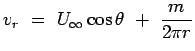
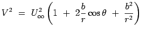
The velocity components for this flow are given by

$$v_r = U_\infty \cos \theta + {m \over {2 \pi r}}$$ (4.94)

$$v_\theta = -U_\infty \sin \theta$$ (4.95)

$$V^2 = U_\infty ^2 \left( 1 + 2 {b \over r} \cos \theta + {b^2 \over r^2} \right)$$ (4.96)

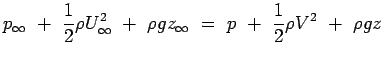
If the pressure in the free stream is $p_\infty$ it follows from Bernoulli Equation that,

$$p_\infty + {1 \over 2} \rho U_\infty ^2 + \rho g z_\infty = p + {1 \over 2} \rho V^2 + \rho g z$$ (4.97)

which enables us to calculate the pressure. Usually in aerodynamic applications involving significant velocities and pressures any contribution due to elevation changes is negligible. The equation for pressure assumes a simple form,

$$p_\infty + {1 \over 2} \rho U_\infty ^2 = p + {1 \over 2} \rho V^2$$ (4.98)

It is left as an exercise for the student to show that the maximum velocity over the surface of the body occurs at the location $\theta = 63^0$ and is approximately equal to $1.26 U_\infty$.

(c) Aerospace, Mechanical & Mechatronic Engg. 2005
University of Sydney