|
Aerofoil Section Analysis using 2D panel
methods,
incorporating 1D corrections for boundary layer flow
SOFTWARE
DOWNLOADS
The prediction of aerodynamic properties of most aerofoil
sections can be obtained relatively accurately using two
dimensional panel method analysis. The solutions will be
primarily inviscid flow predictions. However, with the
introduction of some simple one-dimensional boundary layer
theory, the inviscid solutions can be corrected due to small
viscosity effects. This allows estimation of lift, drag and
pitching moment coefficients for sections were there are only
small effects due to flow separation or friction.
The solution is obtained by two separate calculations,
It is possible to iterate between the results of these two
solutions until a final converged solution is obtained but in
many cases problems may arise due to the number of iterations
required and the possibility of an unstable iteration. A
reasonable result is generally obtained by just using a single
pass of the solution parts.
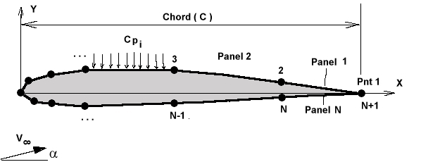
PART 1 : 2D Inviscid panel method
A potential flow solution of any general aerofoil section can
be modelled by descretising the surface contour using singularity
panels. Many different techniques are possible but for the
program used here, the following configuration has been employed
for the panel modelling,
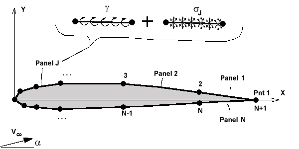
Each panel ( j ) is a straight line segment between
surface contour points (j and j+1). Along the
panel, a source distribution of constant strength ( )
is applied. This distribution strength varies from panel to
panel. As well, along each panel is a constant vorticity
distribution ( )
is applied. This distribution strength varies from panel to
panel. As well, along each panel is a constant vorticity
distribution ( ).
The vorticity is the same on each panel around the contour and
produces the required circulation for the lifting section. ).
The vorticity is the same on each panel around the contour and
produces the required circulation for the lifting section.
As the geometry of the section and
the freestream flow conditions (
 -- velocity ,
 -- angle of attack ) are set, the requirement will be to
define boundary condition equations in order to determine the
necessary distribution strengths (
and
, j = 1 to N (number of panels) ), for an accurate model
of the problem.
-- angle of attack ) are set, the requirement will be to
define boundary condition equations in order to determine the
necessary distribution strengths (
and
, j = 1 to N (number of panels) ), for an accurate model
of the problem.
A boundary condition of no flow through surface (
 )
can be applied at the center of each panel. This produces N
equations in N+1 unknowns. In order to correctly solve for the
extra unknown vorticity, a Kutta condition must be applied at the
trailing edge. )
can be applied at the center of each panel. This produces N
equations in N+1 unknowns. In order to correctly solve for the
extra unknown vorticity, a Kutta condition must be applied at the
trailing edge.
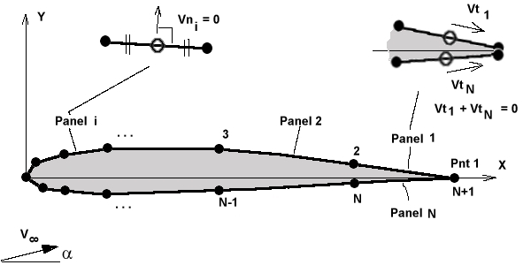
For a single panel (i) the boundary
condition will be applied as,
 at
Panel (i) at
Panel (i)
where the coefficient, ,represents
the influence of the source component on panel (j) on the
control point on panel (i) and , ,represents
the influence of the source component on panel (j) on the
control point on panel (i) and ,
 ,
represents the influence of panel (j) vortex component on
the control point of panel (i). ,
represents the influence of panel (j) vortex component on
the control point of panel (i). represents
the freestream influence. All coefficients are functions of the
geometry of the section, function (x,y), due to
orientation and spacing of panels. represents
the freestream influence. All coefficients are functions of the
geometry of the section, function (x,y), due to
orientation and spacing of panels.
The Kutta condition, equation N+1, can be applied
in terms of trailing edge tangential velocities,

thus
 . .
Written interms of influence coefficients
contributing to the sum of trailing edge tangential velocities,
this becomes,
 . .
This gives a system of linear equations which allow
the solution for the required distribution strengths to be found.
Once the distribution strengths (
 )
have been calculated, surface tangential velocities at the center
of each panel can be calculated ( V ) and then surface
pressure coefficients, )
have been calculated, surface tangential velocities at the center
of each panel can be calculated ( V ) and then surface
pressure coefficients,
The lift coefficient can be calculated assuming a
small angle of attack as the integration of surface pressure
coefficient acting in the y-direction, ie. projected on the x
axis.
Solutions only need to be calculated for one or two
angles of attack as the lift curve will be linear. Stall and
boundary layer effects are not predicted by the first part of the
process.
PART 2 : 1D
Boundary Layer Theory.
Once the surface velocities have been predicted, it
is possible to start some simple calculations for the viscous
surface effects and drag cofficient.
APPLICATION
: 2D Panel Code Computer Program.
The following program accepts
ASCII data files which consist of a list 2-D aerofoil section
coordinates. The format of these aerofoil input data files is the
same as that produced by the NACA
section generation program.
|