Thin Aerofoil Section Theory (2-D)

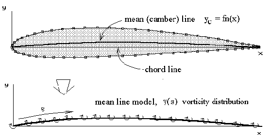
A simple solution for general two-dimensional aerofoil sections can be obtained by neglecting thickness effects and using a mean-line only section model. For incompressible, inviscid flow, an aerofoil section can be modelled by a distribution of vortices along the mean line.

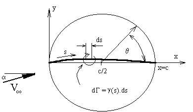
The vortices along the mean line form a continuous vorticity distribution. The assumed distribution function is shown in the following equation. This function is Glauert's approximation and is based on Joukowski transformation results and obeys the Kutta condition with zero vorticity at the trailing edge.

The vorticity distribution is given as a function of the angular variable (q ) which is related to chordwise position (x) as follows,

where c is the chord length. Note that chordwise position (x) is used instead of distance along the mean line (s). For typical aerofoils with small camber, the difference is negligible.

The magnitude of the vortex distribution strength must be calculated to complete the mathematical model. For these thin cambered plate models a boundary condition of zero flow normal to the surface is applied in order to create an equation that can be solved for the required strengths.

The vorticity distribution function has two parts. The first is a constant coefficient (A_o) multiplied by a tangent function which describes the variation due to angle of incidence effects. The second part is a Fourier sine series which will account for variation due to camber. Finally, both parts are scaled by multiplying by the freestream velocity.

Given an aerofoil geometry, freestream velocity and angle of incidence, the magnitude of the coefficients (A₀,A₁,A₂,....) is to be found by solving the condition of zero flow normal to the surface. This condition can be formulated in terms of horizontal and vertical flow velocity components.

thus

The ratio of vertical to horizontal velocity at the surface must equal the surface (mean line) gradient.

The flow horizontal and vertical velocities are made up of freestream and vortex induced components.

and

where u_i and v_i are the horizontal and vertical velocities induced by the vortex distribution.

Both of these components will be much less than the freestream velocity so for small angles of incidence the horizontal vortex induced component can be neglected. If small angle assumptions are made for the incidence, the boundary condition equation becomes

The velocity induced vertically (v_i) at any point on the mean line can be found by summing up the effects of small individual segments (ds) of the vorticity distribution.

where x is the location at which the induced velocity is being calculated and s is the chordwise location of the vortex element. Substituting this result for induced velocity into the boundary condition equation gives

The solution for coefficients (A₀,A₁,A₂,...) can now be obtained from this equation. The solution is based on Glauert's integral method. The equation is summed along the chord line to find initially coefficient A₀. It is then scaled by cosine multiples and again summed along the chord. Each scaled integration will yield one coefficient.

along chord line gives

And similarly integrating the Boundary Condition multiplied by cos nq gives

Once the vorticity coefficients are found the lift of a small element of the vortex line can be predicted from the Kutta-Joukowski law. The complete lift is found by summing all elements of lift from leading to trailing edge.

because of the sector symmetry of the vorticity function only the first two coefficients (A₀,A₁) will contribute directly in this integration. Thus lift coefficient can be found as follows

By summing elements of vortex lift which are multiplied by a moment arm based on their distance from the 1/4 chord point, the pitching moment coefficient can be found.

The following program accepts ASCII data files which consist of a list 2-D aerofoil section coordinates. The format of these aerofoil input data files is the same as that produced by the NACA Section generation program. There is an initial header line, followed by a line giving the number of data points used to describe the aerofoil and then pairs of surface coordinate points (x,y). The order of surface points is anti-clockwise, starting at the trailing edge, going back over the upper surface around the nose and then forward along the underside back to the trailing edge.

From the surface coordinate data file, the program calculates a set of mean-line coordinate points to use as the mathematical thin-aerofoil model. For a given angle of incidence, coefficients A₀,A₁,A₂,.... are calculated using the above equations. Since the mean-line model is a set of straight line segments connecting data points, all integration is done numerically.

The program can then predict C_L versus angle and C_m(1/4c) for the specified aerofoil section. The result is a thin-aerofoil, inviscid flow approximation and therefore has no viscous boundary layer effects. In particular, no stall prediction is possible and the predicted drag coefficient is zero.

Executable Program : Thin-Aerofoil (2-D) Theory(250k)

Reference: "Aerodynamics for Engineering Students" E.L.Houghton & P.W.Carpenter, 4th ED, Edward Arnold, London, 1993.

 Return to Table of Contents