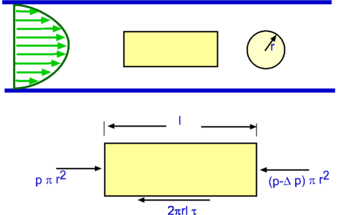
Figure 7.6: Control Volume analysis of pipe flow.
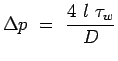
Let us consider a small element of flow of length l around the centreline of the pipe in the fully
developed region as shown in Fig.7.6. The acceleration on the element is zero as the
flow is fully developed. The only
forces acting upon the fluid element considered are the shear
force and the one due to pressure. Let  be the shear stress
acting and pressure at the left hand end of the element be p.
Assuming a pressure drop of be the shear stress
acting and pressure at the left hand end of the element be p.
Assuming a pressure drop of  over the length l the
pressure acting upon the right hand end is over the length l the
pressure acting upon the right hand end is
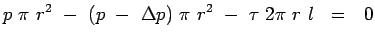
 . A
force balance gives, . A
force balance gives,
| |
 |
|
which on simplification gives, |
|
| |
 |
(7.3) |
The above relation establishes that pressure gradient in
equilibrium with shear stress is the one that keeps the flow
moving. Let us examine Eqn.7.3 in detail. We have which is independent of the radial distance r. Of course l
is independent of r. Consequently  should also be
independent of r. Hence, should also be
independent of r. Hence,
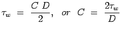
where C is a constant. Then at the walls of the pipe( i.e., r = D/2, where D is the diameter of the pipe) we have,
where  is the wall shear stress, i.e., shear stress at the
wall. is the wall shear stress, i.e., shear stress at the
wall.
Accordingly, our equation for shear stress Eqn.7.4 becomes
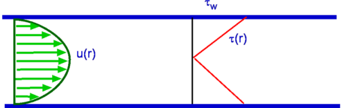
Figure 7.7: Velocity and shear stress distribution in a pipe flow.
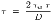
Thus we see that the shear stress varies linearly over the
cylinder radius (see fig.7.7).
Combining Eqns. 7.3 and 7.6 we get,
The Eqn. 7.7 tells us that for a long slender cylinder
( ) even a small shear stress can produce a big pressure
drop. ) even a small shear stress can produce a big pressure
drop.
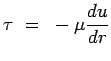
Note that we have so far not made any assumption about the flow
being laminar or turbulent. The equation 7.7 is therefore
very general. In the rest of the present derivation we will
assume a laminar, Newtonian flow for which we have,
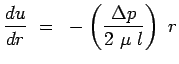
Let us now combine Eqn. 7.3 with Eqn. 7.8 to obtain
an equation for the velocity profile for a laminar flow in a pipe,
integrating this equation we have,
| |
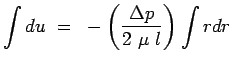 |
|
| |
|
i.e., |
 |
(7.10) |
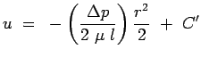
where C' is the constant of integration. This is evaluated from
the boundary condition that velocity is zero at the wall. Thus,
| |
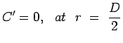 |
|
giving |
|
| |
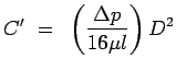 |
|
leading to |
|
i.e., |
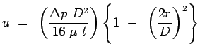 |
(7.11) |
Note that at the centreline we have the maximum velocity. Denoting
it by Vc, we have
| |
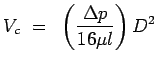 |
|
leading to |
|
i.e., |
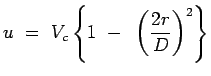 |
(7.12) |
This is the parabolic velocity profile for a laminar flow through
a pipe.
Subsections
(c) Aerospace, Mechanical & Mechatronic Engg. 2005
University of Sydney
|