
Code_Aster
®
Version
7.4
Titrate:
Dynamic nonlinear algorithm of Code_Aster
Date
:
06/07/05
Author (S):
F. VOLDOIRE, G. DEVESA, Mr. AUFAURE
Key
:
R5.05.05-B
Page
:
1/44
Manual of Reference
R5.05 booklet: Transitory or harmonic dynamics
HT-66/05/002/A
Organization (S):
EDF-R & D/AMA
Manual of Reference
R5.05 booklet: Transitory or harmonic dynamics
Document: R5.05.05
Dynamic non-linear algorithm of Code_Aster
(operator
DYNA_NON_LINE
)
Summary:
The operator
DYNA_NON_LINE
[U4.53.01] of Code_Aster gets busy for the non-linear dynamic analysis of
structures by a direct integration in time. Non-linearities can come from the behavior of
material, of the connections (contact-friction), or great geometrical transformations (great displacements
and great rotations).
The organization of
DYNA_NON_LINE
are strongly connected with that of the non-linear quasi-static operator
STAT_NON_LINE
[R5.03.01]. A priori, all relations of behavior developed within the framework of
STAT_NON_LINE
function in that of
DYNA_NON_LINE
.
One presents here the general formulation of the non-linear dynamic problem in order to specify the hinges
between the purely dynamic aspects and those already treated in other operators or formulations
available in Code_Aster: management of the boundary conditions, the couplings fluid-structure, of
damping, of calculation in relative reference mark, then properties of the diagram of numerical integration temporal, which
work out yourself independently of any relation of behavior. It is exposed how the aforementioned is articulated with
the algorithm of Newton to treat material and geometrical non-linearities. Code_Aster proposes two
implicit schemes in effective times in term of precision and stability: that of Newmark and method
“of modified average acceleration” (known as “HHT” in the control
DYNA_NON_LINE
). One gives some
consultings and choice for a good use.

Code_Aster
®
Version
7.4
Titrate:
Dynamic nonlinear algorithm of Code_Aster
Date
:
06/07/05
Author (S):
F. VOLDOIRE, G. DEVESA, Mr. AUFAURE
Key
:
R5.05.05-B
Page
:
2/44
Manual of Reference
R5.05 booklet: Transitory or harmonic dynamics
HT-66/05/002/A
Count
matters

Code_Aster
®
Version
7.4
Titrate:
Dynamic nonlinear algorithm of Code_Aster
Date
:
06/07/05
Author (S):
F. VOLDOIRE, G. DEVESA, Mr. AUFAURE
Key
:
R5.05.05-B
Page
:
3/44
Manual of Reference
R5.05 booklet: Transitory or harmonic dynamics
HT-66/05/002/A
1 Notations
U
field of continuous absolute displacement
K
,
nor
K
stamp rigidity, stamps tangent
M
stamp inertia
R
vector of the interior forces
L
vector second member of loadings (linear form)
abso
L
,
iner
GR.
L
,
anél
L
second members respectively due to an absorbing border, the inertial terms
non-linear in great rotations of beam, with chainings anelastic (coming from
variables of control: temperature…)
C
stamp damping
Q
stamp assembled deformation
T
V
…
transposed of a vector
V
: dual linear form…
T
;
T
time; no time
parameter of the diagram of temporal integration method
(HHT)
,
parameters of the diagram of temporal integration of NEWMARK
increment of various sizes during the pitch of time
virtual variation of a field;
increment of various sizes during iterations of correction
I
;
N
;
J
index of the pitch of time; index of the iteration of NEWTON; index of component
,
µ
parameters of LAGRANGE: reactions of connection, reactions of contact
U U U
,
&, &&
vector ddl successive displacement and derivative compared to time
P
vector ddl of disturbances of fluid pressure barotrope
potential vector ddl of disturbances of fluid displacement barotrope
configuration: vector position:
X y Z
,
and possibly vector rotation, and others
fields parameterizing the system
&
temporal derivative of the configuration
compared to time: speed of traverse and
possibly angular velocity
&&
temporal derivative of
&
compared to time
: acceleration of translation and
possibly angular acceleration
Convention of the repeated indices:
()
()
U T
U T
dk
K
dk
K
K
=

Code_Aster
®
Version
7.4
Titrate:
Dynamic nonlinear algorithm of Code_Aster
Date
:
06/07/05
Author (S):
F. VOLDOIRE, G. DEVESA, Mr. AUFAURE
Key
:
R5.05.05-B
Page
:
4/44
Manual of Reference
R5.05 booklet: Transitory or harmonic dynamics
HT-66/05/002/A
2 non-linear Dynamics
: space discretization of
continuous problem
To solve a non-linear problem of dynamics requires to describe the equations first of all of
continuous problem, then to present their space discretization, here in finite elements, and finally to describe
method of temporal integration, associated the processing of material non-linearities and
geometrical.
2.1
Discretization of the linear problem of dynamics
One notes
U
the field of absolute displacements compared to the configuration of reference, and
parameterized by the moment
T
, pertaining to space refines acceptable fields
adm
V
.
The direct method consists in solving the problem resulting from the discretization by finite elements of
formulation in displacement.
The discretization of the virtual variation of the kinetic energy gives the virtual work of the forces
of inertia, in a field
0
adm
V
v
, directing vector space of
adm
V
:
()
U
V.M.
v
.
U
U
&&
&&
&
T
D
D
=
=
2
2
1
Discretization of the virtual variation of the work dissipated in viscosity (damping brought by one
dependence of the stresses according to speeds of deformation) is:
U
V.C.
v
.
U
.v
U
&
&
&
T
D
C
D
C
=
=
One specifies with [§2.2.1] how the operator of damping
C
is built in
DYNA_NON_LINE
.
The discretization of the variation of elastic energy into linear gives the virtual work of the efforts
interiors:
() ()
() ()
V.K.U
v
.A.
U
U
.A.
U
T
D
D
=
=
2
1
Lastly,
L
designate the second member resulting from the discretization of the virtual work of the external forces.
In linear elasticity, that thus leads to consider the hyperbolic différentio-algebraic system
according to, for the ddl
U
, with the initial conditions:
()
()
=
=
=
+
+
0
0
0
0
:
R
I
U
U
U
U
L
K.U
U
C.
U
Mr.
U
&
&
&
&&
T
T
N
To find
accompanied by boundary conditions.
The initial conditions are provided to the algorithm by the key word
ETAT_INIT
(operands
DEPL
and
QUICKLY
).

Code_Aster
®
Version
7.4
Titrate:
Dynamic nonlinear algorithm of Code_Aster
Date
:
06/07/05
Author (S):
F. VOLDOIRE, G. DEVESA, Mr. AUFAURE
Key
:
R5.05.05-B
Page
:
5/44
Manual of Reference
R5.05 booklet: Transitory or harmonic dynamics
HT-66/05/002/A
If the initial state results from a simulation in or not-linear linear statics, one does not take into account
of initial speed, and displacement, as well as the variables of state (forced, variables intern),
are extracted from the result of this simulation at the starting moment considered.
The dynamic system of balance becomes unstable if one can find a pulsation
complex which
that is to say not real positive for which one can cancel the determinant of:
-
+
+
2
M
C K
I
.
2.2 Discretization
problem
of non-linear dynamics
One places oneself now within a non-linear mechanical framework.
Virtual work is noted
(
) ()
D
T
v
.
U
U
,
, &
of deformation (known as also of the forces intern)
non-linear problem of mechanics, which is written after discretization:
(
)
()
(
)
(
)
U
C.
U
U
.
U
Q
V.
U
C.
U
U
R
V.
&
&
&
&
+
=
+
T
T
T
T
T
,
,
)
,
,
(
where one voluntarily distinguished the linear viscous forces (operator
C
) of the other forces
interns. In the case of small displacements, the operator of deformation assembled
Q
T
is constant
(and definite on the initial configuration confused with the deformation).
The mechanical assessment of energy is written:
(
) ()
+
=
D
T
D
v
.
U
U
v
.
U
v
L.
,
, &
&&
The stress field
at the moment
T
is written in a general way
)
,
,
,
,
(
H
Z
U
U
T
&
, if one notes
Z
field of variables of control, such as for example
T
the field of temperatures, and
H
history
passed of the structure until the moment
T
. For the incrémentaux behaviors, the history is
the whole of the states (fields of displacements, stresses and variables intern) at the previous moment.
In the linear case (cf [§ 2.1]), one leads to
()
U
C.
K.U
U
C.
U
U
R
&
&
&
+
=
+
,
, where
K
is the matrix of
elastic rigidity of the structure and
C
the matrix of damping.

Code_Aster
®
Version
7.4
Titrate:
Dynamic nonlinear algorithm of Code_Aster
Date
:
06/07/05
Author (S):
F. VOLDOIRE, G. DEVESA, Mr. AUFAURE
Key
:
R5.05.05-B
Page
:
6/44
Manual of Reference
R5.05 booklet: Transitory or harmonic dynamics
HT-66/05/002/A
2.2.1 Damping
It is permissible to use discrete elements on which one makes carry a behavior
of damping via a matrix acting on the ddl, cf [U4.42.01], but damping can too
to relate to the massive models or of structures. The operator of damping
C
of the latter can
to be in definite Code_Aster in two ways in
DYNA_NON_LINE
, cf also [R5.05.04], [U2.06.03]:
1) a total way on a basis of clean modes
()
K
established as a preliminary on the structure
rubber band, expressed on the basis of “physical” modeling by finite elements. One defines thus
a coefficient by selected mode. The key word:
AMOR_MODAL
of the operator
DYNA_NON_LINE
allows
to provide him the base of modes and the coefficients damping reduced (according to the assumption of
BASILE). Indeed, depreciation is in experiments given by modal analysis
on resonances.
Displacements
U
are thus projected on the modes to obtain their co-ordinates
generalized:
K
T
K
=
.U
. The matrix of modal damping is:
(
)
(
)
K
T
K
modal
K
=
K
.
.C
K
C
with
K
K
T
K
K
K
modal
=
.K.
C
.
2
where
K
is the factor
of modal damping to the pulsation
K
and
K
K
T
K
K
=
.K.
is the stiffness generalized of
mode
K
. Unfortunately this matrix can have a very full profile and make expensive (them
matrices
C
and
K
not having the same profile), as one will see it with [§ 3.1], his integration
in the first member: one will then choose to treat these forces of modal damping
()
T
U
C.
&
-
with the second member by an explicit diagram.
2) a total/local way known as viscous damping proportional (according to the assumption of
RAYLEIGH) starting from the matrices of elastic stiffness
K
and of mass
M
. The parameters are
given by material on the finite elements of the model (key words
AMOR_ALPHA/AMOR_BETA
of
the control
DEFI_MATERIAU
). The matrix of viscous damping is
M
K
C
+
=
. It
is diagonalisable on the basis of real mode clean, which makes possible to make a calculation
transient on modal basis by uncoupling the modes: to see [R5.06.04]. This formulation, in
linear, led to a damping ratio related to the frequency
F
:
()
F
F
4
/
+
=
. In
non-linear case, this evaluation does not have any more course.
The coefficients in practice are adjusted
,
so that damping
that is to say almost
uniform in the range
[
]
2
1
, F
F
of frequency of interest for the studied structure. From where thus of
reasonable manner:
(
)
2
1
2
F
F
+
=
and
2
1
2
1
.
.
2
.
F
F
F
F
+
=
If the law of behavior of material is non-linear dissipative, the choice of the parameters
of damping
relate to the range where the structure remains almost elastic.
Moreover, it should be noted that, during the integration of non-linearities (cf [§ 3.2] and [§ 3.3]),
Produced Code_Aster of the tangent matrices and viscous damping proportional becomes:
M
K
C
+
=
T
the matrix of mass
M
initial, as for it, being preserved. This makes delicate the interpretation of
the effect of damping proportional. In particular in the event of appearance of eigenvalues
negative of the matrix
T
K
(for example in the event of damage of material),
damping can become negative and reinforce instabilities!

Code_Aster
®
Version
7.4
Titrate:
Dynamic nonlinear algorithm of Code_Aster
Date
:
06/07/05
Author (S):
F. VOLDOIRE, G. DEVESA, Mr. AUFAURE
Key
:
R5.05.05-B
Page
:
7/44
Manual of Reference
R5.05 booklet: Transitory or harmonic dynamics
HT-66/05/002/A
2.2.2 Inertia
One notes
(
)
U
U
U
V.M
&&
&,
,
T
after discretization, virtual work
&&.
U v
D
inertias of
system.
One notes
M
the matrix of mass of the system in small transformations. In great rotations of
structure (such as for example the beams, cf [R5.03.40]), this virtual work is a function
non-linear of
()
U
T
and of its derivative temporal (specifically of the degrees of freedom of
rotation); one thus reveals the usual term of acceleration with a non-linear correction:
(
)
()
(
)
U
U
U
L
U
.
U
M
U
U
U
M
&&
&
&&
&&
&
,
,
,
,
iner
GR.
+
=
. In the other cases,
(
)
()
U
.
U
M
U
U
U
M
&&
&&
&
=
,
,
, which can
to vary if the geometry is reactualized, or who is constant in small displacements.
2.2.3 Connections
In practice, one can have bilateral or unilateral conditions of connection, or connections of the type
“impedance” or “absorbing”, cf [R4.02.05].
Bilateral connections
The bilateral connections are written in the form of the following relation:
()
T
D
U
B.u
=
. Fields of
virtual displacements kinematically acceptable check:
0
B.v
=
. The operator
()
B U
can
to depend on the configuration in the presence of great displacements by reactualization with each pitch
time.
They are perfect: they do not dissipate energy. They are connections “holonomists”, where
speed
&U
does not intervene. These connections are in general dualisées by Code_Aster, cf [R3.03.01].
Unilateral connections
The mechanical system object of simulation by finite elements can come into contact (connections
unilateral) with “obstacle”, which is a solid which one knows a priori the movement, from where
definition of a play
()
D
0
T
. The unilateral connections (for example the unilateral contact) are written on
configuration at any moment
T
:
() ()
()
T
T
0
D
.u
U
With
(nonpenetration or checking that effective play
remain positive or null in any configuration). The operator
()
With U
can depend on the configuration in
presence of great displacements per reactualization with each pitch of time.
One will consider only connections “holonomists”, type
()
WITH U, T
=
0
, which utilizes only them
values of the degrees of freedom
()
U T
and time explicitly if the obstacle is mobile. One
will not consider connections “non-holonomists”, for example of the bearing type without slip, which
utilize speed explicitly and are written
()
()
0
,
,
2
1
=
+
T
T
U
With
U
.
U
With
&
,
With
2
and dependence
direct in time being present only if it there a mobile obstacle.
If the obstacle is motionless, the connection as such will be explicitly independent of time (one says
also “scleronomist”).
These “loads of contact” are defined by the operator
AFFE_CHAR_MECA
. The presence of connections
unilateral requires to define speeds of the solid in a particular functional space in order to ensure
the existence of solutions of the system of dynamics. Indeed, at the time of the moments (countable)
of impact, speeds
()
&U T
-
and
()
&U T
+
can not coincide. It is necessary to guarantee it
result that the data (loading, equations of connections) check a property of analycity, which is
acquired in practice with the selected discretization by finite elements (see [bib6]).

Code_Aster
®
Version
7.4
Titrate:
Dynamic nonlinear algorithm of Code_Aster
Date
:
06/07/05
Author (S):
F. VOLDOIRE, G. DEVESA, Mr. AUFAURE
Key
:
R5.05.05-B
Page
:
8/44
Manual of Reference
R5.05 booklet: Transitory or harmonic dynamics
HT-66/05/002/A
One does not introduce a priori a relation constitutive of the impacts (dissipative behavior in rebound
simple, expressed using a coefficient of normal restitution
[]
E
0 1
,
), expressed on the differentials
speeds of the two points in impact:
()
()
()
()
(
)
&
&
&
&
_
_
_
_
U
U
U
U
2
1
2
1
norm
norm
norm
norm
T
T
E
T
T
+
+
-
-
=
-
-
This type of behavior is introduced usually indeed to treat the contact-impact of body
rigid, whereas numerical modeling with deformable solids makes it possible to represent
directly the vibratory behavior under the shock and material non-linearities. But it is
possible to add in the modeling of the discrete elements of contact-shock placed on the interface in
contact, fitted with the law
DIS_CHOC
, which brings a dissipation of damping (to condition of
to suppose small movements…).
One can associate with the unilateral connections a behavior of friction (criterion of COULOMB), which
dissipate energy in relative slip of surfaces in contact.
One refers sometimes to the fact that the dynamic coefficient of friction is lower than that
measured into quasi-static (adherence). That comes owing to the fact that in dynamics from the vibrations high
frequency on the normal reaction appear and weaken the value of the threshold of friction of
COULOMB. One would thus not need to provide two values of coefficients to Code_Aster,
since one modelizes the deformable solids in contact-friction (on the condition of being able to simulate these
vibrations high frequency…).
It is known that dissipation is a condition necessary for the existence of theoretical solutions to
problem of dynamics with impact. Use of the diagram HHT, to see [§ 5], which introduces
numerical dissipation can prove to be necessary.
Local dissipative connections
Specific relations (like
DIS_CONTACT
,
DIS_CHOC
) are conceived to treat certain types
dissipative specific connections, acting directly on the ddls of discrete elements of the system,
to see [R5.03.17]. They constitute a law of behavior in generalized forces function of
generalized displacements integrated like the whole of the internal forces
R U U
(,
&,)
T
structures
studied.
Absorbing connections
The “absorbing” connections of the type, cf [R4.02.05], make it possible to simulate the “filtering” of a part
dynamic response, by preventing the exit of diffracted waves, with the profit of an “incidental” field
on a border of the model: to see it [§ 2.6]. They introduce damping terms of the type
()
With
U
abso
&
on a border of the solid considered.
2.2.4 Discretized dynamic problem
The dualisation of the boundary conditions of DIRICHLET
)
(
T
D
U
B.u
=
and of the unilateral conditions
conduit after discretization to define the unknown factors at any moment
T
:
(
)
U,
, µ
, where
represent them
“multiplying of LAGRANGE” of the boundary conditions of DIRICHLET [R3.03.01], and
µ
represent the “multipliers of L
AGRANGE
” of the unilateral conditions.
The non-linear dynamic problem is written, with the initial conditions [R3.03.01], [R5.03.50]:

Code_Aster
®
Version
7.4
Titrate:
Dynamic nonlinear algorithm of Code_Aster
Date
:
06/07/05
Author (S):
F. VOLDOIRE, G. DEVESA, Mr. AUFAURE
Key
:
R5.05.05-B
Page
:
9/44
Manual of Reference
R5.05 booklet: Transitory or harmonic dynamics
HT-66/05/002/A
To find the trajectory
()
U T
:
(
) (
)
()
()
()
()
()
=
=
=
-
=
=
+
+
+
+
0
0
0
0
0
0
0
,
0
,
.
,
,
,
,
U
U
U
U
.
D
A.U
D
U
With
U
B.U
L
A.
B.
U
C.
U
U
R
U
U
U
M
&
&
&
&
&&
&
T
T
J
J
T
T
T
T
J
J
J
D
T
T
µ
)
(
µ
µ
éq 2.2.4-1
L
represent the vector of the external forces (mechanical loadings). These forces can
to depend on time and space. It is supposed that, like the connections, they depend on way
regular of the parameters, which ensures the existence of the solution of the problem (theorem of
CAUCHY). One can consider “following” forces
()
T
,
U
L
, for example pressure, if one takes
in account changes of geometry.
The vector
B.
T
be interpreted like the opposite of the reactions of support to the corresponding nodes (
B
is the linear operator expressing the passage to the degrees of freedom of the supports). The vector
A.µ
T
be interpreted like the nodal forces due to the contact (
With
is the linear operator expressing it
passage to the degrees of freedom of the areas in contact).
The analysis of stability of the dynamic system of balance [éq 2.2.4-1] is more complex than into linear,
but a sufficient condition of loss of stability is the possibility of finding a pulsation
for
which one can cancel the determinant of:
T
T
I
K
C
M
+
+
-
2
, definite on the operators
tangent, at the moment considered.
2.2.5 Conditions
initial
Initial conditions
U U
0
0
,
&
are provided to the code by the key word
ETAT_INIT
(operands
DEPL
and
QUICKLY
).
If the initial state results from a simulation in or not-linear linear statics, displacement, as well as
variables of state (forced, variables intern), are extracted from the result of this simulation, and
initial speed by defect is supposed to be null.
2.2.6 Implicit temporal piloting of external loadings
In general, loads, defined in
AFFE_CHAR_MECA
or
AFFE_CHAR_MECA_F
, are of type
“
FIXE_CSTE
” if their intensity and direction are known a priori.
One can as consider as a share of the external stresses is controlled (standard “
FIXE_PILO
”),
i.e. its intensity is parameterized:
F
imp
pilo
and/or
U
imp
pilo
, and controlled by a relation
scalar, expressed on a node (or groups nodes), on the solution:
()
()
P
T
P
U
= =
~
, this
last being implicit. As it is seen, this equation refers to the time, which contrary to
the statics where it is only used to give a chronology on the increments of load, has a physical role
in dynamics. One will have to thus ensure oneself of the precise significance of temporal piloting.

Code_Aster
®
Version
7.4
Titrate:
Dynamic nonlinear algorithm of Code_Aster
Date
:
06/07/05
Author (S):
F. VOLDOIRE, G. DEVESA, Mr. AUFAURE
Key
:
R5.05.05-B
Page
:
10/44
Manual of Reference
R5.05 booklet: Transitory or harmonic dynamics
HT-66/05/002/A
One thus adds in the non-linear system [éq 3.1-7] this last equation which will be solved with
others by the iterative method of NEWTON. One cannot control the forces of gravity, of
centrifugal force, of LAPLACE, the thermal or anelastic deformations.
One will be able usefully to refer to [R5.03.80].
2.3
Taking into account of a prestressed initial state
If the dynamic problem to solve “follows” an initial mechanical state, two main situations
are offered to us:
·
{}
1
one wishes to calculate displacements
U
and dynamic stresses starting from the state
“virgin” no initial,
·
{}
2
one wishes to calculate displacements
U
and dynamic stresses in “differential”
starting from a preloaded state.
In the first situation
{}
1
, the weather is advisable to be during the calculation of the static state as a preliminary,
possibly non-linear (material, great transformations), precondition to dynamics.
Thus, if the structure has a non-linear behavior, one must proceed directly in dynamics
non-linear, after having evaluated the state initial by simulation in statics, possibly non-linear
(with the operator
STAT_NON_LINE
), and the field of displacement is evaluated since the beginning of
the history. It can be necessary to take into account the variations of geometry. Information
necessary to describe the initial state (results of a preceding simulation via the concept result
EVOL_NOLI
or mechanical fields necessary:
DEPL
,
SIGM
,
VARI
) are provided by the key word
ETAT_INIT
, for example if one is within the framework of an incremental behavior (
COMP_INCR
),
to see [U4.51.03].
The initial state can be also obtained by a simulation in “very slow” dynamics, by having care of
to put a “slow” slope of dependence at time on the static efforts applied, like one
strong damping (physical, cf [§ 2.2.1] or/and numerical cf [§ 5]). This manner of proceeding has
the advantage of injecting so much into the operator of the phase of prediction [éq 3.2.1-4] of the algorithm of
NEWTON, that in that of the phase of correction [éq 3.3-1] of the terms
$K
coming from the matrix from
mass and of that of damping, to establish the static mechanical state. That is invaluable in
situations of contact-friction, damage… to improve convergence.
The second situation
{}
2
relate to the case of a structure which underwent a preloading
thermomechanical “ordinary”, leading to a state of linear elastic balance. If one measures
by
U
displacement starting from this preloaded state, which generated a state of stresses
1
, then
the elastic deformation energy is supplemented by a geometrical term of stiffness:
() ()
()
(
)
.U
K
K
V.
v
U
.
v
.A.
U
G
T
D
D
+
=
+
1
One then assembles simply the matrices
K
and
K
G
, and the resolution in dynamics is carried out
linear, as with [§ 2.1]. That can be for example the case of a seismic study on a stopping
arch. With
DYNA_NON_LINE
, it is necessary to provide by the key word
ETAT_INIT
, the field of
stresses
SIGM
result of the preloaded state and to specify with the key word
DEFORMATION
under
COMP_INCR
the taking into account of the non-linear terms of deformation.
It is frequent that the contribution of
K
G
that is to say negligible: one can then be satisfied with an analysis
dynamics on the basis of completely virgin initial state. It will be also noted that the calculation of the matrix
K
G
is not available for all the finite elements proposed by Code_Aster.

Code_Aster
®
Version
7.4
Titrate:
Dynamic nonlinear algorithm of Code_Aster
Date
:
06/07/05
Author (S):
F. VOLDOIRE, G. DEVESA, Mr. AUFAURE
Key
:
R5.05.05-B
Page
:
11/44
Manual of Reference
R5.05 booklet: Transitory or harmonic dynamics
HT-66/05/002/A
2.4
Coupled problems vibroacoustic fluid-structure
One will be able for more details to refer to the documents [R4.02.02], [R4.02.04], [R4.02.05].
One considers the small movements approaches eulérienne of a compressible true fluid it,
possibly bathing a wall of a solid structure. The fluid is known as barotrope:
·
one considers small irrotational disturbances around the initial state (hydrostatic):
R
R
R
U
U
U
fl
fl
fl
=
+
0
,
p
P
P
+
=
0
and
+
=
0
F
, index 0 indicates the permanent part of
fields),
·
the law of behavior of the fluid gives the stresses “
fluctuating
”
:
(
)
Id
Id
Id
fl
U
C
C
p
R
div
2
0
0
2
0
=
-
=
-
=
,
·
fluid speeds derive from a potential
=
=
&
r&
R
fl
fl
U
v
and are modelized using
fields
()
p,
: pressure fluctuating and potential of displacement, which are not
independent bus
:
&
&
p
C
= -
0 02
(by combining equation of continuity and law of
behavior).
It is admitted that one does not consider fluctuating forces of volume
RF
being exerted on the fluid.
The dynamic balance of the fluid is written:
0r
&&r
=
+
fl
F
p
U
(equation of linearized Euler), which is valid
for a not-heavy fluid compressible or weighing incompressible; on the other hand for a heavy fluid
compressible the approaches eulérienne and Lagrangian do not coincide even into small
movements: this case is not treated by Code_Aster.
The dynamic balance of the fluid will be written in variational form under the action of a pressure
fluctuating
p
imp
imposed on part of the border. In harmonic mode, dynamic balance
fluid results in the variational formulation of the equation of Helmholtz.
Code_Aster has a symmetrized formulation, to see [R4.02.02], with elements
()
,
P
noting it
vector of the ddl of pressure and fluctuating potential to describe the disturbances in the fluid,
knowing that
0
0
R
&&
=
+
p
. An equation in
P
solves dynamic balance in the field
fluid, that in
translating the equation of derived continuity combined with the fluid law of behavior.
Boundary conditions in
P
and
supplement the system of equations to describe the evolutions
fluid. Thus, on a border
p
F
_
fluid field, a fluctuating pressure can be
applied:
()
T
imp
P
P
=
, however because of the formulation
()
,
P
, one must also impose one on it
condition on
:
()
()
T
T
imp
=
, checking
()
()
T
T
imp
imp
P
=
&&
0
.
As one considers a border common fluid-structure
FS
, where the normal is defined
RN
outgoing of the structure field towards the fluid, the loading of wall of the fluid is coupled with
displacement of the structure. Normal displacements are continuous:
(
)
N
.
U
N
.
U
U
R
R
R
R
R
St
fl
fl
=
+
0
on
FS
,
Ru
fl
0
indicating the permanent part of fluid displacement. By using the fluid potential, one
a:
N
.
U
N
.
R
r&
R
&
St
=
on
FS
. In a dual way, the vectors forced are continuous:
N
.
N
R
R
=
-
p
on
FS
. The structure thus receives the loading fluctuating of the fluid
:
()
-
FS
dS
p
N
.
v
R
R
.

Code_Aster
®
Version
7.4
Titrate:
Dynamic nonlinear algorithm of Code_Aster
Date
:
06/07/05
Author (S):
F. VOLDOIRE, G. DEVESA, Mr. AUFAURE
Key
:
R5.05.05-B
Page
:
12/44
Manual of Reference
R5.05 booklet: Transitory or harmonic dynamics
HT-66/05/002/A
If one considers a free face (subjected to a constant pressure), also treated of description
eulérienne, to see [R4.02.04], one notes by
Z
(and
Z
ddl associated after discretization) altitude
fluctuating (small) of the free face
SSL
and the fluctuation in pressure eulérienne in the fluid
check:
(
)
0
0
=
-
SSL
zdS
gz
p
, in any virtual altitude
Z
. It is the only consequence of
gravity which one can take account in this formulation.
In addition, one can need to take into account an artificial border with an infinite medium
(which must treat the condition of radiation ad infinitum): Code_Aster proposes finite elements of border
absorbing (paraxial or anechoic elements), to see [R4.02.05]. As they bring a priori one
term in derived third of time, because of the introduction of the field
, one prefers to treat it with
the aid of a transformation into a not-symmetrical term in
P
&
who will be deferred to the second member, of
explicit manner.
On the whole one obtains the différentio-algebraic semi-discrete equations of the coupled problem:
free
surfing
fluid
fluid
structure
St
Z
fl
F
Z
T
Z
fl
fl
T
FS
T
fl
FS
.
=
+
+
0
0
0
L
Z
P
U
K
0
0
0
0
0
0
0
0
0
Q
0
0
0
0
K
Z
P
U
0
0
0
0
0
0
With
0
0
0
0
0
0
0
0
C
Z
P
U
0
M
0
0
M
H
M
M
0
M
0
0
0
M
0
M
&
&
&
&
&&
&
&&
&&
éq 2.4-1
accompanied by the initial conditions:
()
U
U
T
0
0
=
,
()
0
0
U
U
&
&
=
T
,
()
0
0
P
P
=
T
,
()
0
0
=
T
and
()
0
Z
=
0
T
,
and of the boundary conditions:
()
imp
T
U
U
=
on the edge
U
S
_
structure, the possible ones
unilateral conditions, and
()
()
T
T
imp
P
P
=
with
()
()
T
T
imp
=
, checking
()
()
T
T
imp
imp
P
=
&&
0
on
edge
p
F
_
fluid.
Note:
It is noted that in the non-linear case, one replaces in [éq 2.4-1] the term
K.U
by the forces
non-linear interns
(
)
T
,
,
,
Z
U
U
R
&
.
The various operators are:
·
matrices
K
, M, C
defined higher for the solid structure,
·
Q
fl
is the matrix built from
F
qd
p
C
.
1
2
0
0
, which has the physical direction of one
elastic energy of the fluid,
·
H
fl
is built from
-
F
D
.
0
, and described the fluid transport of mass,
·
M
fl
is built from
F
qd
C
.
1
2
0
, and described the inertia of the fluid,
·
M
FS
is built from
()
-
FS
dS
N
.
v
R
R
.
0
(
RN
is the normal of the field
structure towards the fluid), and described the mass throughput eulérien with the interface fluid-structure,

Code_Aster
®
Version
7.4
Titrate:
Dynamic nonlinear algorithm of Code_Aster
Date
:
06/07/05
Author (S):
F. VOLDOIRE, G. DEVESA, Mr. AUFAURE
Key
:
R5.05.05-B
Page
:
13/44
Manual of Reference
R5.05 booklet: Transitory or harmonic dynamics
HT-66/05/002/A
·
With
F
is built from
0
p D
F
.
, and the operator absorbing border indicates,
acting on
&P
, modifying the equation in
absorbing wall: the elements (model
3d_FLUI_ABSO
) absorbents die-symmetrize the system resulting from the formulation
()
,
P
and one goes
to defer this term to the second member, who will be noted
abso
L
, by temporal discretization
clarify with each iteration, to see the § 3,
·
K
Z
is the “stiffness” of free face, built from
SSL
zdS
gz
.
0
,
·
M
Z
comes from the work of the fluctuating pressure in free face, built from
SSL
dS
Z
.
0
,
·
the term
L
St
contains, inter alia loadings, the effect of the exerted hydrostatic pressure
by the fluid on the structure.
In short, the taking into account of a fluid field in fluctuating evolution barotrope, interacting
with the structure results in considering in the non-linear dynamic system [éq 2.2.4-1] enriched on
particular ddls
()
,
P
and
Z
:
·
an operator of inertias
()
MR. U U
.
&&
nouveau riche by:
=
Z
P
U
0
M
0
0
M
H
M
M
0
M
0
0
0
M
0
0
Z
P
U
M
&&
&&
&&
&&
&&
&&
&&
&&
Z
T
Z
fl
fl
T
FS
T
fl
FS
fs
;
·
an operator of interior forces
(
)
R U U
,
&
nouveau riche by:
=
Z
P
U
K
0
0
0
0
0
0
0
0
0
Q
0
0
0
0
0
Z
P
U
K
Z
fl
fs
;
·
a second member enriched by the carryforward with the second member by temporal discretization
clarify
P
With
&
F
-
on the ddls
.
The fluid must remain in small movements (basic assumption of this modeling), but one can
to consider great movements of the structure, bathed by the fluid, via a reactualization of
geometry
X
X
U
+
(via the key word
COMP_INCR
, operand
DEFORMATION
:
“PETIT_REAC”
,
valid if one considers small rotations) borders
FS
, which makes recompute the term
M
FS
but also all others since the field
F
evolved/moved; scalar fields
()
,
P
are then
simply transported to identical on the reactualized geometry. See also case-test FDNV100
[V8.03.100].

Code_Aster
®
Version
7.4
Titrate:
Dynamic nonlinear algorithm of Code_Aster
Date
:
06/07/05
Author (S):
F. VOLDOIRE, G. DEVESA, Mr. AUFAURE
Key
:
R5.05.05-B
Page
:
14/44
Manual of Reference
R5.05 booklet: Transitory or harmonic dynamics
HT-66/05/002/A
2.5 Taking into account of laws of viscous behavior and
damping
A law of viscous behavior, to see [R5.03.08], is translated like an elastoplastic law by one
evolution of the work of the interior forces
R U U
(,
&,)
T
. Thus, while bringing a damping
“physical” in dynamic balance, it does not produce a direct taxation at the end
of damping
C U
.
&
dynamic equilibrium equation, but however in an indirect way if one
chose a damping of Rayleigh (cf [§ 2.2.1]) via the matrix of tangent stiffness of the diagram
of integration.
Indeed with a law of viscous behavior, the tensor of the deformations comprises a part
rubber band, a thermal part, a anelastic part (known) and a viscous, deviatoric part
(diverter of the stresses noted
~
), for example checking:
()
(
)
eq
eq
v
E
v
has
HT
E
early
T
T
.
With
~
2
3
,
,
G
=
=
+
+
+
=
&
For the relation of viscous behavior
LEMAITRE
, the function
G
is explicit, but it is not
always the case. After implicit discretization in time, the viscous flow is:
()
v
eq
v eq
eq
T
T
=
+
-
3
2 G
,
,
~
One can also adopt an semi-implicit diagram, which seems to give better results:
()
v
eq
v eq
eq
T
T
T
=
+
+
+
+
+
-
-
-
-
-
3
2
2
2
2
2
2
G
,
,
~
~
After solution of a local non-linear equation per elimination of
v
to calculate
(
)
eq
eq
=
+
-
, one thus obtains the stress at the end of the pitch of current time
=
+
-
.
2.6
Equations of “relative” motion [R4.05.01]
In several applications, in particular in seism, one wishes to calculate the field directly of
displacement of the structure deduced from the movement of “drive” coming from displacements
imposed
()
U
D
T
supports of the structure.
One notes then
U
has
the absolute displacement of the structure:
U
U
U
+
=
ent
has
,
ent
U
being displacement
of drive (for example,
ent
U
can be an incidental field: it is then called “displacement
pseudo-statics “)) ; it can be rigid body (case
MONO_APPUI
), but not necessarily (case
MULTI_APPUI
).

Code_Aster
®
Version
7.4
Titrate:
Dynamic nonlinear algorithm of Code_Aster
Date
:
06/07/05
Author (S):
F. VOLDOIRE, G. DEVESA, Mr. AUFAURE
Key
:
R5.05.05-B
Page
:
15/44
Manual of Reference
R5.05 booklet: Transitory or harmonic dynamics
HT-66/05/002/A
And one calls
U
the “relative” displacement (called thus by abuse language if
ent
U
is not
rigid body).
Indeed coding (RCC-M, ASME…) introduced the distinction between “primary stresses” due
with the vibratory movement “relative” and “secondary stresses” due to the vibratory movement
of “drive”. The relevance of this distinction disappears a priori obviously as soon as one considers
a non-linear behavior of material.
If one deals with the problem of interaction with the ground (which is an infinite half space) in seism by
example, the field of relative displacement
U
check:
()
lim
X
U X
=
0
: only the incidental field
ent
U
is
perceptible ad infinitum it is the seismic data of loading. One uses to define this loading
of displacement imposed the control
AFFE_CHAR_MECA
and the key word factor
ONDE_PLANE
, on one
border given of the mesh considered.
In this case of problem of interaction with the ground, one does not know a priori displacement
of “drive” directly applied to the structure, since it results from the coupled total answer:
also the case
MULTI_APPUI
does not have it a direction.
On the other hand, not being able to simulate in finite elements with Code_Aster the field in all the half
infinite space (ground), one is led to place “absorbing” borders, cf [R4.02.05], at the edge of
mesh of ground. The virtual work associated these absorbing borders, of outgoing normal
N
, is
treated as a second member (for the finite elements paraxial absorbents of command 0), because it is
integrated explicitly in the diagram of temporal integration (cf [§3]) of
DYNA_NON_LINE
.
associated linear form is worth:
(
)
() ()
()
(
)
-
+
=
abso
dS
ent
abso
ent
abso
ent
ent
abso
v
.
U
With
.n
U
U
With
v
.
U
U
U
L
&
&
&
&,
,
éq 2.6-1
After discretization, one deduces the second member:
(
)
()
ent
abso
T
ent
T
abso
T
ent
ent
abso
T
U
V.A
U
V.
U
V.A
U
U
U
V.L
&
&
&
&
&
.
.
,
,
-
+
=
éq 2.6-2
Note: case of a problem with interaction fluid-structure:
For a structure undergoing of imposed displacements, in the presence of fluid interaction
structure, where the fluid field is not directly related to the “support” imposing the signal
of drive, it is possible to solve the dynamic system of balance in term of
“relative” displacement
U
fluid structure and variables
()
,
P
“absolute” and of dimension of
free face of the fluid
Z
“absolute”, cf [§ 2.4]. Indeed, one can show that
(
)
0
P
=
ent
ent
,
and
0
Z
=
ent
, on the basis of [eq 2.4-1]. One will be able to refer to [R4.02.05].
One will not be able to consider such a type of decomposition field of “drive” field
“relative” in the event of loadings of fluctuating the pressure type imposed on a wall of the fluid field.
One seeks to exploit this distinction in the discrete non-linear dynamic system [éq 2.2.4-1]
to simplify the taking into account of imposed displacements
()
U
D
T
.
Code_Aster
®
Version
7.4
Titrate:
Dynamic nonlinear algorithm of Code_Aster
Date
:
06/07/05
Author (S):
F. VOLDOIRE, G. DEVESA, Mr. AUFAURE
Key
:
R5.05.05-B
Page
:
16/44
Manual of Reference
R5.05 booklet: Transitory or harmonic dynamics
HT-66/05/002/A
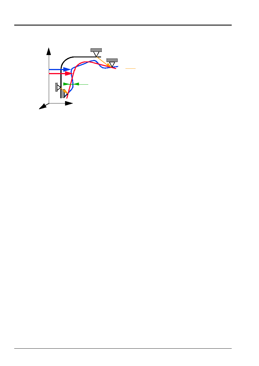
absolute movement
U
has
movement of drive
U
relative movement
U
S
imposed displacement of the supports
U
U
ent
(R has)
U
has
U
ent
All the conditions of connection, to see [éq 2.2.4-1], are not necessarily conditions
of “drive” by the supports:
()
T
D
has
S
U
.U
B
=
; one notes by
0
.U
B
=
has
L
conditions of
connections which one wishes to impose directly on displacement
U
has
structure (for example of
connections intern like “
3d_POU
”…) and
L
parameters of associated LAGRANGE. One considers
thus thereafter these two families:
S
B
for the movements of “drive” by the supports and
L
B
for the bilateral connections “ordinary”.
If the supports are in a finished number (what will be the case in any case after discretization), one notes
V
E
vector space of the fields of displacements of the “involved” structure
ent
U
, of dimension
finished
NR
S
, that one will define hereafter. The conditions of DIRICHLET are broken up
()
U
D
T
, on one
base
()
X
ks
displacements of the supports:
()
()
U
X
D
dk
ks
T
U T
=
,
K
NR
S
=
1
traversing all them
“degrees of freedom involved” by the supports.
One builds a “raising elastostatic”, i.e. a base of
V
E
starting from the solutions
linear elastic statics of the structure under only basic imposed displacements
()
X
ks
supports (no loading in imposed force). After discretization by finite elements, that returns to
to solve
S
NR
K
=
1
problems of elastostatic (matrix of stiffness
K
):
To find
(
)
K
K
L
S
K
,
,
such as
=
=
=
+
+
0
B
X
B
0
B
B
K
K
L
ks
K
S
L
L
T
S
S
T
K
K
K
.
.
.
.
.
éq
2.6-3
One calls “static modes” these
NR
S
solutions
K
(well informed via the operand “
MODE_STAT
” of
DYNA_NON_LINE
). They are calculated as a preliminary by the operator
MODE_STATIQUE
[U4.52.04] with
the option
MODE_STAT
.
One necessarily has with [éq 2.6-3]:
0
.
=
+
K
S
S
T
K
T
.
X
.K
L
L
,
S
NR
K
=
1
,
L
.
The field of displacements of the “involved” structure
ent
U
, after discretization by finite elements,
is thus described by
()
K
K
ent
ent
T
U
=
U
, checking in particular
()
ks
K
D
ent
S
T
U
X
U
B
=
.
on
supports, traversing the discrete subspace
V
E
, of the “degrees of freedom involved” by the supports.

Code_Aster
®
Version
7.4
Titrate:
Dynamic nonlinear algorithm of Code_Aster
Date
:
06/07/05
Author (S):
F. VOLDOIRE, G. DEVESA, Mr. AUFAURE
Key
:
R5.05.05-B
Page
:
17/44
Manual of Reference
R5.05 booklet: Transitory or harmonic dynamics
HT-66/05/002/A
The discrete subspace
V
E
is thus generated by the base
()
K
. One necessarily has:
()
()
U T
U T
K
ek
dk
=
,
The degrees of freedom of displacements of the “involved” structure thus are directly given by
the value of
()
U
D
T
.
Having characterized the discrete subspace
V
E
starting from the static modes, after discretization,
let us study a field of displacement
W
structure, kinematically acceptable unspecified, but
no one on the supports:
B W 0
S
.
=
and checking the “ordinary” connections
0
W
B
=
.
L
. Under the terms of
[éq 2.6-3], one necessarily has:
0
W
B
W
W.B
W.X
W.B
B
W.
B
W.
W.K
=
=
=
=
+
+
.
,
0
.
.
0
.
.
.
S
K
L
T
ks
T
K
S
T
L
L
T
T
S
S
T
T
K
T
K
K
that
such
From where simply:
0
W
B
0
W
B
W
W.X
W.K
=
=
=
=
.
.
,
0
0
.
L
S
ks
T
K
T
and
that
such
éq
2.6-4
The elastic operator of stiffness
K
being definite positive (having eliminated the rigid modes of body), one
note that any field of absolute displacement
W
has
kinematically acceptable of the structure,
after discretization, can be written by single decomposition:
W
W W
has
E
=
+
on the sum of the additional subspaces
V
V V
has
E
=
éq
2.6-5
with
V
E
generated starting from the static modes
()
K
, and
V
containing the fields known as “ddls active”
such as
B W 0
S
.
=
(null on the supports). One calls
V
the discrete subspace of the “degrees of
freedom credits “.
For a loading of the type
MONO_APPUI
, the static modes are the rigid modes of body of
structure:
0
K
=
K
.
, checking the “ordinary” connections
0
B
=
K
L
.
.
If the loading is
MULTI_APPUI
, static modes
()
K
are unspecified.
This decomposition on two additional subspaces
V
V V
has
E
=
of any field
kinematically acceptable built using the operator of elasticity
K
is applicable in all
non-linear evolution of the structure, including with shocks…, provided that connections
bilateral remain the same ones during the history.

Code_Aster
®
Version
7.4
Titrate:
Dynamic nonlinear algorithm of Code_Aster
Date
:
06/07/05
Author (S):
F. VOLDOIRE, G. DEVESA, Mr. AUFAURE
Key
:
R5.05.05-B
Page
:
18/44
Manual of Reference
R5.05 booklet: Transitory or harmonic dynamics
HT-66/05/002/A
Let us exploit this decomposition and project the non-linear dynamic problem now
[éq 2.2.4-1] separately on the subspace
V
then on the subspace
V
E
, while exploiting [éq 2.6-3].
The result is simplified (a little only) bus
B W 0
S
.
=
(from where the “active ddls” do not work
in the reactions of the supports supports
B
S
),
B
0
L
K
.
=
(from where the static modes do not work
in the reactions of connection
B
L
),
B
X
S
K
ks
.
=
:
To find
U
U
U
has
E
=
+
,
S
,
µ
L
,
such as:
()
(
)
(
)
()
(
)
(
)
(
)
(
)
()
(
)
(
)
(
)
(
)
(
)
(
) ()
(
)
()
=
+
=
+
=
-
+
+
=
=
-
-
+
=
+
+
+
+
+
+
+
-
-
+
=
+
+
+
+
+
+
+
=
0
0
0
0
0
0
0
,
0
)
(
,
,
)
,
,
(
,
,
,
,
)
,
,
(
,
,
U
U
U
U
U
U
.
D
U
U
A.
D
U
U
A.
0
.U
B
0
.U
B
A.
.
.
X
U
U
U
L
L
.
U
U
U
.R
U
U
.C.
U
U
U
U
U
U
.M
W
A.
W.
.
B
W.
U
U
U
L
L
W.
U
U
U
W.R
U
U
W.C.
U
U
U
U
U
U
W.M.
U
&
&
&
&
&
&
&
&
&
&&
&&
&
&
&
&
&
&
&
&
&&
&&
&
&
L
L
T
T
J
T
K
T
T
T
T
T
U
E
E
J
J
E
E
L
S
T
K
T
S
ks
T
E
E
abso
K
T
E
K
T
E
K
T
E
E
E
K
T
T
T
L
L
T
T
E
E
abso
T
E
T
E
T
E
E
E
T
D
E
µ
µ
µ
µ
V
éq 2.6-6
It is noted that that is rather intricate.
We with the dynamic problem restrict initially where operators of inertia
M
and of forces
interior
R
are linear, and in absence of absorbing borders:
(
)
0
U
U
U
L
=
&
&,
,
E
E
abso
.
One makes the assumption in Code_Aster that:
C U
0
.
&
E
=
, including in multi-support (whereas that is not
exact that in mono-support, where the static modes are the rigid modes
K
0
.
K
=
without deformation).
That amounts neglecting the contribution of displacements of drive of the structure to
viscous damping.

Code_Aster
®
Version
7.4
Titrate:
Dynamic nonlinear algorithm of Code_Aster
Date
:
06/07/05
Author (S):
F. VOLDOIRE, G. DEVESA, Mr. AUFAURE
Key
:
R5.05.05-B
Page
:
19/44
Manual of Reference
R5.05 booklet: Transitory or harmonic dynamics
HT-66/05/002/A
Static modes
K
checking [éq 2.6-3], the system [éq 2.6-6] is restricted with:
()
()
(
)
()
()
()
()
(
)
()
(
)
(
)
(
) ()
(
)
()
=
+
=
+
=
-
+
+
=
=
=
-
-
=
+
+
+
-
-
-
=
+
+
0
0
0
0
0
0
0
,
0
)
(
U
U
U
U
U
U
.
D
U
A.
D
U
A.
0
.U
B
0
.U
B
U
A.
.
.
X
.L
.K.
U
.C.
U
.M.
W
U
W.M.
A.
W.
.
B
W.
W.L
W.K.U
U
W.C.
U
W.M.
&
&
&
&
&&
&&
&&
&
&&
L
L
L
L
T
T
T
U
J
T
T
U
T
U
K
T
T
U
T
U
T
E
E
J
J
K
K
D
K
K
D
L
S
K
K
D
E
T
K
T
S
ks
T
K
T
K
T
D
K
T
D
K
T
E
T
T
T
L
L
T
T
T
T
T
T
µ
µ
µ
µ
V
éq 2.6-7
One notes on the first of these equations [éq 2.6-7], that thanks to the made assumptions, one can
to restrict to solve a dynamic problem on the field of “relative” displacement
U
, having
locked the degrees of freedom on the supports (
B U 0
S
.
=
), with the proviso of providing it as a preliminary
term
T
E
W MR. U
.
&&
, as well as the static modes
()
K
.
The object of the operator
CALC_CHAR_SEISME
[U4.63.01] is precisely to calculate the term
E
T
U
M
W
&&
.
.
-
,
transformed into a concept of the type
“load
”, using the operator
AFFE_CHAR_MECA
[U4.25.01].
One can also simply introduce a load of unit “gravity” into the wanted direction, and
amplified by the temporal signal of acceleration. The advantage is to exploit the data directly in
accélérogramme (for example produced starting from a spectrum), without having to twice integrate it in time
with uncertainties which this operation generates. One can produce the stresses directly known as
“primary” induced by dynamics in “relative movement”.
This advantage is lost if unilateral connections are present, since the condition
()
(
)
WITH U
D
.
()
+
U T
T
dk
K
0
ask the value of
()
U T
dk
to be expressed correctly, except if
one with the chance that the movement of drive does not have a component on the interface where play of
the unilateral connection is calculated!
The second equation of [éq 2.6-7] provides the reactions on the supports
S
(the remainder being given
by the resolution of the problem in “relative” displacement
U
); but it is noted there too that it is
necessary to know
()
U T
dk
.
It is the same thing if one wants to reconstitute the complete solution for postprocessing in
stresses with their “secondary” contribution known as, related to
()
U
E
dk
K
U T
=
.
Now one considers the dynamic problem of a structure interacting with a ground (medium
“infinite”), source of an incidental seismic wave, cf [R4.05.01] and [R4.02.05]. One is necessarily
within a framework “
MONO_APPUI
”, where the static modes are the rigid modes of the structure, from where:
K
0
.
K
=
and
T
K
.C U
.
&
=
0
. One thus uses elements of absorbing border, and the term
(
)
L
U U U
abso
E
E
,
&, &
is present in [éq 2.6-7]. The incidental wave is provided directly by the signal

Code_Aster
®
Version
7.4
Titrate:
Dynamic nonlinear algorithm of Code_Aster
Date
:
06/07/05
Author (S):
F. VOLDOIRE, G. DEVESA, Mr. AUFAURE
Key
:
R5.05.05-B
Page
:
20/44
Manual of Reference
R5.05 booklet: Transitory or harmonic dynamics
HT-66/05/002/A
()
U
D
X T
R,
. One thus builds the terms of [éq 2.6-2], as well as the term
T
E
W MR. U
.
&&
.
system [éq 2.6-7] becomes:
()
(
)
()
()
(
)
()
(
)
()
()
T
T
T
T
T
abso
E
T
E
T
T
L
L
T
T
T
E
T
K
D
T
K
T
K
abso
E
T
K
E
T
ks
S
T
K T
E
dk
K
S
T
U T
T
K
U T
W.M U
W.C U
W.K U
W.L
W.A
U U
W.U
W.B
W.A
W.M U
W
.M U
.L
. With
U U
. U
X.
. With
U
B
.
&&
.
&
.
.
&
&
&
.
.
.
&&
.
& & &&
.
&
&
&
.
+
+
=
+
-
+
-
-
+
=
+
-
+
-
-
=
0
0
µ -
µ
V
L
L
()
(
)
()
(
)
(
)
(
) ()
(
) ()
.
.
.
()
.
& &
&
U
0
B U
0
WITH U
D
WITH U
D
U U
U
U U
U
=
=
+
+
=
+
=
+
=
L
dk
K
dk
K
J
J
E
E
U T
T
J
U T
T
T
0
0
0
0
0
0
0
0
µ
,
-
.µ
éq 2.6-8
Let us return now to the non-linear general problem [éq 2.6-6]. It is noted that the first
equation on the “active” degrees of freedom comprises necessarily a coupling with the field
()
U
E
dk
K
U T
=
in the operator of inertia as in that of internal forces. One thus must,
in accordance with the diagram of temporal integration and non-linear resolution, developed with [§ 3],
to reconstitute calculation at every moment the value of absolute displacement
U
U
U
has
E
=
+
, them
stresses…
In conclusion, one can deal with the dynamic problem moving relative (by admitting that them
forces of damping depend only on him):
·
if one is in
MONO_APPUI
or
MULTI_APPUI
, provided that the behavior is linear in
small transformations, without absorbing border, with unilateral conditions such as
the plays are modified by the movement of drive, only the fluid field
that is to say directly not charged, and with a loading of imposed acceleration, cf [éq 2.6-7];
·
if one is in
MONO_APPUI
, with an unspecified behavior and absorbing border,
with unilateral conditions such as the plays are not modified by the movement
of drive, and with a loading of imposed acceleration.
If not, one can only deal with the dynamic problem moving absolute.

Code_Aster
®
Version
7.4
Titrate:
Dynamic nonlinear algorithm of Code_Aster
Date
:
06/07/05
Author (S):
F. VOLDOIRE, G. DEVESA, Mr. AUFAURE
Key
:
R5.05.05-B
Page
:
21/44
Manual of Reference
R5.05 booklet: Transitory or harmonic dynamics
HT-66/05/002/A
3
Diagram of temporal integration: diagram of NEWMARK and
method of
NEWTON
The mechanical problem to analyze being modelized in finite elements, according to the step described with
[§ 2], one calculates the fields of displacements, speeds and accelerations with the nodes in a continuation
discrete of moments of calculation
T T
T
T
T
I
I
NR
1 2
1
,
,
K
K
-
:
{}
T
I
I NR
1
.
The user of
DYNA_NON_LINE
can currently choose between two implicit temporal diagrams with
two pitches: that of NEWMARK (1959) or its alternative known as “modified average acceleration”, of
HILBER-HUGUES-TAYLOR (HHT, 1977): to see the paragraph [§5]. The state of the structure being known with
the moment
T
I
-
1
, one deduces his state at the moment from it
T
I
by a method of prediction-correction.
Note:
One must note that Code_Aster does not propose method multi-field in time and space, which
would allow to define a diagram by area in the studied solid.
3.1 Diagram
of
NEWMARK
One presents here this diagram in his conventional form ([bib1] and [bib2]) relating to a movement of
translation or of small rotation. For great rotations of elements of structure [bib3], the formulas
are more intricate, but they in the same way make it possible to bring up to date speed and acceleration
angular according to the increase in displacement, which is in this case vector-rotation.
One notes hereafter by
configuration, i.e. the parameter setting of the system by the ddl of
finite elements: displacements and rotations
U
, pressure
P
, potential
…
The diagram of NEWMARK rests on the following developments of the vector configuration function
time, when
and
are two parameters:
(
)
()
()
(
) ()
(
)
(
)
T
T
T
T
T
T
T
T
T
+
+
-
+
+
+
&&
&&
&
2
2
1
2
2
éq
3.1-1
(
)
()
(
) ()
(
)
(
)
T
T
T
T
T
T
T
+
+
-
+
+
&&
&&
&
&
1
éq
3.1-2
The equation [éq 3.1-1] is also written with [éq 3.1-2]:
(
)
()
(
) ()
(
)
(
)
(
) ()
T
T
T
T
T
T
T
T
T
&&
&
&
2
2
2
-
+
+
+
-
+
+
These parameters
and
are provided respectively via the operands
ALPHA
and
DELTA
key word
NEWMARK
of
DYNA_NON_LINE
.
See it [§ 4] for the characteristics of the diagram according to the values of these parameters.
The hooks with the second members of the equations [éq 3.1-1] and [éq 3.1-2] are averages
balanced
()
T
&&
and of
(
)
T
T
+
&&
.
In practice these expressions are not usable because one will have to express the values at the moment
T
T
+
from those at the moment
T
.
Code_Aster
®
Version
7.4
Titrate:
Dynamic nonlinear algorithm of Code_Aster
Date
:
06/07/05
Author (S):
F. VOLDOIRE, G. DEVESA, Mr. AUFAURE
Key
:
R5.05.05-B
Page
:
22/44
Manual of Reference
R5.05 booklet: Transitory or harmonic dynamics
HT-66/05/002/A
The equation [éq 3.1-1] gives:
(
)
(
) ()
[
]
()
()
()
()
T
T
T
T
T
T
T
T
T
T
T
T
T
&&
&
&&
&&
&
&&
2
1
1
1
2
1
2
1
1
2
2
-
-
=
-
+
-
-
+
=
+
éq
3.1-3
And, according to [éq 3.1-2]:
(
)
(
) ()
[
]
() (
)
()
() (
)
()
T
T
T
T
T
T
T
T
T
T
T
T
T
&&
&
&
&&
&
&
2
2
2
2
-
+
-
=
-
+
-
+
-
+
=
+
éq
3.1-4
It is noticed that one cannot have
0
=
, nor
0
=
. With the first pitch of calculation one exploits directly
initial conditions:
()
0
and
()
0
&
. It is necessary too
()
0
&&
, except if
1
=
: to see the remark made with
[§ 3.2].
In the case of great rotations of elements of structure homologous expressions with [éq 3.1-3] and
[éq 3.1-4] are more complex [bib5], but the relations which follow are rather easily
transposable.
During a pitch of time (of
T
with
T
T
+
), where values at the moment
T
are solidified, the equations
[éq 3.1-4] and [éq 3.1-3] the increases speed define
&
and of acceleration
&&
agent with an increase in arbitrary displacement
starting from the position at the moment
T
,
which one will need at the time of the iterations of correction of NEWTON (within the pitch of time, to see it
[§ 3.3]):
T
=
&
éq
3.1-5
2
1
T
=
&&
éq
3.1-6
We place at the moment
T T
I
=
-
1
, and one writes balance [éq 2.2.4-1] after space discretization with
the moment
T
T
T
I
I
=
+
-
1
, possibly with the complementary elements brought in [éq 2.2-6]. One
note
()
I
I
T
U
U
=
degrees of freedom at the new moment
I
T
and by exploiting the terms of the diagram
temporal [éq 3.1-4] and [éq 3.1-3], one leads to the non-linear system of dynamic balance:
(
)
()
(
)
()
=
-
=
-
=
+
+
+
0
,
0
,
)
(
,
,
^
,
,
^
0
0
J
J
I
I
J
I
I
I
D
I
I
I
I
iner
GR.
I
I
T
I
T
I
I
I
J
J
T
T
T
T
µ
)
(
µ
µ
.
D
A.U
D
A.U
U
B.U
U
U
U
L
L
A.
B.
U
U
R
U
K
&&
&
&
éq 3.1-7

Code_Aster
®
Version
7.4
Titrate:
Dynamic nonlinear algorithm of Code_Aster
Date
:
06/07/05
Author (S):
F. VOLDOIRE, G. DEVESA, Mr. AUFAURE
Key
:
R5.05.05-B
Page
:
23/44
Manual of Reference
R5.05 booklet: Transitory or harmonic dynamics
HT-66/05/002/A
with:
(
)
C
M
M
K
K
T
T
fs
fs
+
+
+
=
2
1
^
éq
3.1-8
() ()
()
(
)
(
)
-
+
-
+
+
-
+
+
+
+
+
=
-
-
-
-
-
-
-
1
2
1
1
1
2
1
1
2
1
2
2
.
1
2
2
1
1
^
I
I
I
I
I
I
fs
I
abso
I
I
T
T
T
T
T
T
T
T
T
U
U
U
C
U
U
U
M
M
L
L
L
&&
&
&&
&
éq
3.1-9
Note:
It is noted that the matrix
$K
contributing to the stiffness generalized of the system to solve is
enriched by terms coming from the matrix from mass
M
system (provided that one has
affected a density on all the finite elements of the model) and the matrix
of damping
C
. One will further see than the linearization from the internal forces
(
)
T
I
I
,
, U
U
R
&
also contribute to
$K
. Thus, even if the mechanical system considered comprises modes
rigid, for example in a study where a solid is in free fall, the matrix of mass comes
“to prevent” that the matrix of “stiffness”
$K
is not factorisable. To some extent, they are them
inertias of the solid body (in its rigid modes) which ensures balance with the forces
external, which could not be done into quasi-static.
However, it is observed that the pitch of time
T
appears too. If it is too large, the terms of
mass will not be important enough vis-a-vis those of stiffness, and quasi stamps it risk to be
non-factorisable (“quasi-null pivots”).
Note:
Terms with the exponent
fs
appear if the system contains fluid fields (see
[§ 2.4] and terms coming from the fluid field in [éq 2.4-1]); it is reminded the meeting that it is not envisaged
of fluid loading
fl
L
.
Note:
Contrary to the case of damping of Rayleigh (see [§ 2.2.1]), the matrix of damping
C
does not appear in the matrix
$K
in the presence of modal damping (key word
AMOR_MODAL
),
because in this case, the force
C U
.
&
I
-
1
is built directly without storage of the matrix
C
, and is
deferred to the second member
()
$L T
I
.
The term
abso
L
in the second member appears in the presence of absorbing borders, to see it
[§ 2.6]. It is treated according to an explicit diagram according to the fields solutions with
T
I
-
1
.
Note:
Contrary to
diagram used in thermics, cf [R5.02.01], where the derivative are written of
explicit manner, while the conservation equation is written at one fictitious moment resulting from one
combination with the parameter
values at the moments
1
-
I
T
and
I
T
, dynamic balances
are checked over the moments
1
-
I
T
and
I
T
, while the derivative are combinations
determined by the diagram [éq 3.1-1] and [éq 3.1-2].
Code_Aster
®
Version
7.4
Titrate:
Dynamic nonlinear algorithm of Code_Aster
Date
:
06/07/05
Author (S):
F. VOLDOIRE, G. DEVESA, Mr. AUFAURE
Key
:
R5.05.05-B
Page
:
24/44
Manual of Reference
R5.05 booklet: Transitory or harmonic dynamics
HT-66/05/002/A
It still remains to treat the non-linear terms: internal forces
(
)
R U U
I
I
T
,
&,
and the contribution
non-linear of the inertias in great rotations of structures
(
)
L
U U U
GR.
iner
I
I
I
,
&, &&
(cf [§ 2.2.2]).
At the first moment
T
1
, one sees in [éq 3.1-9] that one needs
U U
0
0
,
&
, provided by the conditions
initial, but also, because of the diagram of NEWMARK, of
&&U
0
: to see the remark made with [§ 3.2].
3.2
Phase of prediction
The system [éq 3.1-7] is non-linear and is integrated, after a prediction of EULER by linearization, with
the aid of an iterative method of NEWTON, as in non-linear statics [R5.03.01]. The calculation of
this prediction can be slightly erroneous, as long as the phase of correction by iterations of
NEWTON [§ 3.3] is able to correct with convergence…
3.2.1 No general time
With the phase of prediction, one exploits the solution with the preceding pitch or the values of the initial state, and one
note the matrix of initial tangent stiffness of the pitch:
(
)
(
)
(
)
(
)
(
)
1
1
1
1
1
1
1
1
1
1
1
,
,
,
,
,
,
1
-
-
-
-
-
-
-
-
-
-
-
+
=
=
-
I
I
I
I
I
I
I
I
I
I
I
T
T
T
T
T
I
D
D
U
U
U
U
U
U
U
U
U
.
Q
.
U
Q
U
R
K
&
&
&
éq 3.2.1-1
These terms (cf [§ 2.2]) are evaluated on the preceding pitch, the first term of the second member of
[éq 3.2.1-1] appearing only in great displacements (
Q
not being then constant).
If the behavior is linear, the matrix
K
I
-
1
is simply the elastic matrix of rigidity
K
of
the structure.
One can also decide to save time calculation not to reactualize this matrix, and of
to take the elastic matrix of rigidity, to see [U4.51.03], key word
NEWTON
, operand
PREDICTION
,
value `
RUBBER BAND
', rather than `
TANGENT
'. If one specifies nothing, the choice by defect made by
Code_Aster is coherent with that done on the iterations of correction of NEWTON described hereafter
with [§3.3].
In addition, in the presence of great rotations (elements of structure: beams…), one must too
to derive the non-linear term from inertia
(
)
I
I
I
iner
GR.
U
U
U
L
&&
&,
,
:
(
)
1
1
1
,
,
1
1
-
-
-
=
-
I
I
I
iner
GR.
I
U
U
U
M
U
L
K
&&
&
éq
3.2.1-2
The matrix
$K
having been established by [éq 3.1-8], this new matrix
1
1
M
K
-
I
is combined with the matrix
$K K
+
-
I 1
, to see below [éq 3.2.1-4].

Code_Aster
®
Version
7.4
Titrate:
Dynamic nonlinear algorithm of Code_Aster
Date
:
06/07/05
Author (S):
F. VOLDOIRE, G. DEVESA, Mr. AUFAURE
Key
:
R5.05.05-B
Page
:
25/44
Manual of Reference
R5.05 booklet: Transitory or harmonic dynamics
HT-66/05/002/A
One defines also the increases in loading
()
$L T
I
from [éq 3.1-9], conditions
imposed
()
I
D
T
U
, and one gathers in
()
I
anél
T
L
dependences of the stresses in function
various parameters or “variables of control”
Z
law of behavior of material
constitutive: such as the temperature…:
()
(
)
(
)
Z
.
Z
U
Q
L
Z
U
U
U
-
=
-
-
-
-
,
,
,
1
1
1
1
.
I
I
I
D
D
T
I
T
I
anél
&&
&
In the presence of modal damping the forces of damping are deferred to the second member.
One adds then to
()
$L T
I
the term corresponding:
1
.
-
-
I
U
C
&
.
The term
()
()
(
)
1
1
1
1
,
,
-
-
-
-
+
-
=
I
I
ent
I
ent
abso
I
F
I
abso
T
T
U
U
U
L
P
With
L
&
&
&
indicate the contribution
integrated into explicit (to simplify) of an absorbing fluid border and an elastic border
absorbing, cf [éq 2.4-1] and [éq 2.6-2].
The increase is noted
()
I
T
L^
,
L^
being defined with [éq 3.1-9]:
() () ()
1
^
^
^
-
-
=
I
I
I
T
T
T
L
L
L
éq
3.2.1-3
One then calculates predictive values for the pitch of time in progress
(
)
U
I
I
I
0
0
0
,
,
µ
:
Prediction
(
)
()
()
()
()
(
)
=
-
=
+
=
+
+
+
+
-
-
0
.
,
0
,
)
(
.
.
^
.
.
^
0
0
0
0
0
0
0
0
0
0
1
1
1
J
I
J
I
I
J
I
I
I
I
D
I
I
anél
I
I
T
I
T
I
I
I
J
J
T
T
T
T
.µ
µ
µ
D
U
With
D
U
With
U
U
B
L
L
With
B
U
K
K
K
M
éq
3.2.1-4
where the prediction is defined
0
1
0
I
I
I
U
U
U
+
=
-
for the new moment
T
T
T
I
I
=
+
-
1
.
If one chose
STAMP
= `
ELASTIQUE'
in the key word
NEWTON
, one does not revalue with each pitch of
time
1
0
0
1
1
1
^
^
M
M
K
K
K
K
K
K
+
+
=
+
+
-
-
I
I
, which avoids the cost of re-assembly and inversion,
but the iteration count of correction increases.
After the establishment of a candidate solution of [éq 3.2.1-4] without checking the criterion of contact, one launches
the algorithm of active stresses to satisfy the conditions of contact: one corrects thus
U
I
I
I
0
0
0
,
,
µ
.

Code_Aster
®
Version
7.4
Titrate:
Dynamic nonlinear algorithm of Code_Aster
Date
:
06/07/05
Author (S):
F. VOLDOIRE, G. DEVESA, Mr. AUFAURE
Key
:
R5.05.05-B
Page
:
26/44
Manual of Reference
R5.05 booklet: Transitory or harmonic dynamics
HT-66/05/002/A
Note: stamp tangent singular:
One checks on [éq 3.2.1-4] whom if the tangent matrix
1
-
I
K
is singular (case of a rigid mode,
of a damaged material, or ductile plate…), dynamics is controlled by the inertias,
and that, the matrix
K^
being in general regular (cf notices made with [§ 3.1]), one finds in spite of
any good a predictor
0
I
U
, provided that precision in the matrix
K^
is not lost
(pivot quasi-no one) because of a choice of pitch of too large time which plays in
2
/
1
T
in
[éq 3.1-8]. It is for example the case in free dynamics of fall.
3.2.2 First pitch of time
If one is with the first pitch of time, a study or a recovery (continuation), the predictor is
calculated differently to take account of the initial state (
U
0
,
0
U
&
,
0
):
(
)
()
()
()
()
(
)
=
-
-
=
-
+
=
+
+
+
+
0
.
,
0
,
)
(
.
.
^
.
.
.
^
0
1
1
0
0
1
0
1
1
0
0
1
0
1
0
1
0
1
1
0
1
0
1
0
1
1
0
0
J
J
J
D
T
anél
T
T
J
J
T
T
T
T
.µ
µ
µ
D
U
With
D
U
With
U
B
X
U
B
Q.
L
L
With
B
U
K
K
K
M
éq
3.2.2-1
with:
() ()
(
)
(
)
-
+
-
+
+
-
+
+
+
+
=
0
0
2
0
0
0
0
2
0
0
2
1
1
2
2
1
2
2
1
1
^
U
U
U
C
U
U
U
M
M
L
L
&&
&
&&
&
T
T
T
T
T
T
T
T
fs
éq
3.2.2-2
and acceleration
0
0
U
&&
evaluated by the preliminary resolution of the system (one simplifies by supposing them
locked connections of contact, the iterations of NEWTON will be given the responsability to correct):
()
()
=
=
-
+
=
+
+
0
0
0
0
0
0
0
0
0
0
0
0
0
A.U
B.U
Q.
L
L
A.
B.
U
Mr.
T
anél
T
T
T
T
µ
&&
éq
3.2.2-3
Note:
It would be more exact to calculate:
()
()
0
0
0
0
0
0
0
0
.
.
.
U
C
Q
L
L
With
B
U
M
&
&&
-
-
+
=
+
+
µ
T
anél
T
T
T
T
,
but to simplify knowing that that will have only little influence on the continuation of the solutions, one
neglect
0
U
C
&
in the second member of [éq 3.2.2-3].

Code_Aster
®
Version
7.4
Titrate:
Dynamic nonlinear algorithm of Code_Aster
Date
:
06/07/05
Author (S):
F. VOLDOIRE, G. DEVESA, Mr. AUFAURE
Key
:
R5.05.05-B
Page
:
27/44
Manual of Reference
R5.05 booklet: Transitory or harmonic dynamics
HT-66/05/002/A
One must note that:
·
the matrix
M
must be invertible: one will have to affect a density on all them
finite elements of the model,
·
it can be necessary to establish by a static calculation (possibly non-linear) the state
of balance under the initial loading, therefore stresses
0
, before the imposition of
initial dynamic conditions
U U
0
0
,
&
. Indeed, if not, acceleration
0
0
U
&&
could be
“excessive” and to lead on a nondesired branch of balance,
·
in the presence of “loads kinematics”, cf [U4.44.03], these last are put at zero with
this stage of calculation of
0
0
U
&&
.
However, certain finite elements do not have mass on all the degrees of freedom, by
example beams with roll
POU_D_TG
precisely on the ddl of roll, or in
fluid coupling/structure. For the vibroacoustic elements of coupling [§ 2.4] indeed, the matrix
of mass of the problem [éq 2.4-1] is not invertible. In these cases, the matrix
M
is not
invertible, and one is satisfied to take a null initial acceleration on the whole of the model and
continuation of the iterations will have to be given the responsability to correct this “good” prediction less. One then will be chosen
small pitch of time to ensure convergence at least the beginning of the transient.
The term
()
0
T
abso
L
is evaluated starting from initial speed
0
U
&
(cf [R4.02.05]).
3.3
Phase of correction by the method of NEWTON
The values are sought
(
)
, µ
U
I
I
I
increments of displacements and parameters of
LAGRANGE since the values
(
)
U
I
-
1
1
1
, µ
I
I
obtained with preceding balance (urgent
T
I
-
1
). One
takes as initial values
(
)
, µ
U
I
I
I
0
0
0
obtained at the end of the phase of prediction, before
to begin the iterations of the method of NEWTON.
With each iteration
N
of NEWTON, one notes by
evolutions leading to the estimate of
increments with convergence of the iterations
:
1
1
1
-
+
+
-
+
=
I
nor
N
I
nor
U
U
U
U
and
I
N
I
N
in
I
+
+
-
=
+
-
1
1
1
(in the same way for
µ
). One must then solve a system allowing of
to determine
(
U
I
N
in
in
+
+
+
1
1
1
,
,
)
µ
, increments of displacements and the parameters of LAGRANGE
since the result
(
)
X
in
in
I
N
, µ
preceding iteration:
Correction (iteration n°
N
)
(
)
()
(
)
=
-
=
-
+
=
+
+
+
+
+
+
+
+
+
+
+
0
.
0
)
(
0
^
^
1
0
1
0
1
1
1
1
1
J
nor
J
I
nor
J
I
nor
nor
N
I
nor
abso
I
nor
T
N
I
T
N
I
N
I
nor
J
J
T
T
µ
µ
µ
.
D
U
With
D
A.U
U
B.
F
L
L
A.
B.
U
K
K
K
M
,
,
éq
3.3-1
Code_Aster
®
Version
7.4
Titrate:
Dynamic nonlinear algorithm of Code_Aster
Date
:
06/07/05
Author (S):
F. VOLDOIRE, G. DEVESA, Mr. AUFAURE
Key
:
R5.05.05-B
Page
:
28/44
Manual of Reference
R5.05 booklet: Transitory or harmonic dynamics
HT-66/05/002/A
with a second member called “residue”, because it tends towards zero to convergence. One notes
(cf balances [éq 2.2.4-1]):
()
(
)
()
(
)
N
I
T
N
I
T
iner
GR.
nor
N
I
nor
T
nor
T
N
I
N
I
N
I
N
I
I
N
I
N
I
µ
A.
B.
L
U
.
U
M
U
C.
.
U
Q
F
U
U
U
U
U
+
+
-
+
+
=
&&
&
&
&&
&
,
,
,
,
éq
3.3-2
The term
()
$L T
I
is defined by [éq 3.1-9], the term
(
)
nor
ent
I
ent
abso
N
I
F
nor
abso
I
1
1
1
,
,
1
-
-
-
-
+
-
=
U
U
U
L
P
With
L
&
&
&
corresponds to the fluid and elastic borders absorbing, which is treated into explicit [éq 2.4-1],
[éq 2.6-2]; the matrix
$K
is given by [éq 3.1-8].
In the presence of modal damping the forces of damping are deferred to the second member.
According to the value given to the key word
AMOR_MODAL
,
REAC_VITE
, one adds to
()
I
T
L^
the reactualized term:
N
I
U
C
&
.
-
, or not reactualized
1
.
-
-
I
U
C
&
.
The matrix
K
in
is the matrix of the tangent linear application of the part “forces intern”
system of non-linear equations [éq 3.1-7]; it is thus worth:
)
,
(
)
,
,
(
)
,
,
(
I
N
I
I
N
I
N
I
I
N
I
N
I
T
méca
I
T
T
N
I
U
U
U
U
U
U
L
U
R
U
F
K
-
=
=
&
&
éq
3.3-3
In the absence of following forces, the last term is null. The following forces can be:
pressure exerted on the edges of solid elements, the loading of gravity for the elements of
cable, the centrifugal force in great displacements, the loading of gravity for all them
modelings
THM
not-saturated porous environments [R7.01.10].
If one considers the reactualization of the geometry (in great displacements), one has more precisely:
()
(
)
()
(
)
)
,
(
,
,
,
,
.
I
N
I
I
N
I
N
I
I
N
I
N
I
T
méca
I
T
T
T
T
N
I
U
U
U
U
U
U
L
U
U
Q
U
U
Q
K
-
+
=
.
&
&
éq
3.3-4
The first term is the contribution of the behavior as in small transformations, with
difference which this contribution is evaluated here in current configuration. The second term is
contribution of the geometry which is not present in small transformations. Within the framework of
reactualization
PETIT_REAC
, this term is not present in the calculation of the tangent matrix.
The matrix
N
I
M
K
is the matrix of the tangent linear application of the part “inertias” of
system of non-linear equations [éq 3.1-7] which is thus worth:
(
)
N
I
N
I
N
I
iner
GR.
N
I
U
U
U
M
U
L
K
&&
&,
,
=
éq
3.3-5
In practice one can use “the true” tangent matrix, but that presents a cost unquestionable calculation
(calculation and factorization), or to be satisfied with a reactualization from time to time: to see in [U4.51.03] it
key word factor
NEWTON
, key word
STAMP
.
Code_Aster
®
Version
7.4
Titrate:
Dynamic nonlinear algorithm of Code_Aster
Date
:
06/07/05
Author (S):
F. VOLDOIRE, G. DEVESA, Mr. AUFAURE
Key
:
R5.05.05-B
Page
:
29/44
Manual of Reference
R5.05 booklet: Transitory or harmonic dynamics
HT-66/05/002/A
Note: stamp tangent singular:
One checks on [éq 3.3-1] whom if the tangent matrix
K
in
is singular (case of a material
damaged, or ductile plate…), dynamics is controlled by the inertias, and that,
stamp
K^
being regular, one finds despite everything good a corrector
U
in
+
1
(as if one were
for example in free situation of fall). However, if the pitch of time is “too high”,
stamp
(
)
N
I
N
I
M
K
K
K
+
+
^
can be badly conditioned and the solvor finds a pivot to him quasi-no one.
After each iteration of NR
EWTON
having established a candidate solution of [éq 3.3-1] without checking the criterion
of contact, one launches the algorithm of active stresses to satisfy the conditions of contact: one
correct thus
U
in
+
1
.
3.4
Update
·
In the case of small rotations, for usual modelings (solid elements,
discrete beams, plates, hulls, elements…), the update is based on the formulas
[éq 3.1-5] and [éq 3.1-6].
+
+
+
+
+
+
+
+
+
+
+
+
1
2
1
1
1
1
1
1
1
1
N
I
nor
nor
nor
nor
nor
nor
nor
nor
nor
nor
nor
T
T
U
U
U
U
U
U
U
U
U
U
U
U
&&
&&
&
=
=
=
=
éq
3.4-1
·
In the case of great rotations of the elements of structure (beams…) the update,
definitely more complex, is indicated in [R5.03.40].
3.5 Criterion
of stop
The criterion of total convergence of the algorithm of NEWTON is identical to that practiced in
STAT_NON_LINE
. It represents the checking of dynamic balance.
At the moment
T
I
, one stops the iterations with the row
N
, as soon as the following inequality is satisfied:
()
()
(
)
()
()
()
-
-
+
-
-
+
+
+
+
nor
T
nor
T
I
anél
I
I
iner
GR.
nor
T
nor
T
nor
N
I
nor
nor
nor
T
T
T
T
N
I
N
I
N
I
µ
µ
A.
B.
L
L
L
L
A.
B.
U
.
U
M
U
C.
.
U
Q
U
U
U
^
^
,
,
&&
&
&&
&
éq
3.5-1
is a tolerance, introduced in data by the user (key word
CONVERGENCE
, operand
RESI_GLOB_RELA
), about 10
4
to 10
6
, and
.
is the standard of the maximum on the ddls.
The denominator of [éq 3.5-1] is a standard of the loading at the moment
T
I
, to which one brings it back
numerator, which is a standard of the forces not (still) balanced.
Code_Aster
®
Version
7.4
Titrate:
Dynamic nonlinear algorithm of Code_Aster
Date
:
06/07/05
Author (S):
F. VOLDOIRE, G. DEVESA, Mr. AUFAURE
Key
:
R5.05.05-B
Page
:
30/44
Manual of Reference
R5.05 booklet: Transitory or harmonic dynamics
HT-66/05/002/A
Just like in statics, one must attach importance to a correct convergence bus if not, them
estimates of interior forces and reactions of contact, checking the relations of behavior and
from connection of contact-friction move away from balance, and it is not an inertia
()
N
I
N
I
U
U
M
&&
.
too much far away from the “exact” value which will be enough to produce with the pitch of time following one
good transitory dynamic response.
One will be able to also employ other criteria of convergence as proposed in
STAT_NON_LINE
.
4
Qualities and defects of the diagram of NEWMARK
4.1
Properties of the diagram of NEWMARK
This paragraph and the following takes again partially certain parts of [bib2]. One will be able too
to consult [bib24] and [bib27].
One defines using the methods of numerical analysis several types of properties for a diagram
of temporal integration. Here their significance:
·
Convergence: the solution tends towards a limit when the pitch of time
T
tends towards 0;
·
Precision: rate of convergence when the pitch of time
T
tends towards 0;
·
Consistency and command of the diagram: the residue is limited by
()
1
+
K
T
(example:
2
=
K
for
regulate trapezoid): a polynomial of command
1
+
K
is integrated exactly;
·
Stability: a finished disturbance of the initial state exaggeratedly does not involve a disturbance
amplified (“numerical explosion”) in a later state; it is necessary that amplification (spectral radius)
that is to say lower than 1: for a diagram of general form
I
I
I
L
WITH
U
+
=
-
1
, one must have
()
1
With
. It is a condition necessary not to diverge! If
()
1
<
With
there is
numerical attenuation.
The error
E
induced by the diagram of NEWMARK [éq 3.1-1], [éq 3.1-2] is given by:
I
T
E
U
&&
6
2
éq
4.1-1
that one can standardize by the vector position
X
or the amplitude
U
. One can also replace in
[éq 4.1-1] the standard
2
L
(
I
U
&&
) by the standard
L
:
()
ki
K
nodes
I
Max
U
U
&&
&&
=
. Today
Code_Aster does not provide the information of this estimator.
The numerical analysis of the diagram of NEWMARK is done on the processing of the equation of the oscillator
linear with a D.D.L., without friction:
0
=
+
kx
X
m &&
éq
4.1-2
Code_Aster
®
Version
7.4
Titrate:
Dynamic nonlinear algorithm of Code_Aster
Date
:
06/07/05
Author (S):
F. VOLDOIRE, G. DEVESA, Mr. AUFAURE
Key
:
R5.05.05-B
Page
:
31/44
Manual of Reference
R5.05 booklet: Transitory or harmonic dynamics
HT-66/05/002/A
The temporal diagrams do not give the exact solution of [éq 4.1-2]:
T
C
T
C
X
sin
cos
2
1
+
=
with
m
K
=
,
1
C
and
2
C
depending on the initial conditions, but an approximate solution:
(
)
[
]
(
)
I
I
I
I
T
C
T
C
T
X
~
sin
~
cos
~
exp
'2
'1
+
-
=
Two errors are thus brought:
·
on the one hand, it is introduced a definite artificial damping by the reduced rate of depreciation
,
who is the decrement logarithmic curve divided by
2
;
·
in addition, the pulsation
corresponding to the exact period
T
is replaced by
pulsation
~
agent at one period
~
T
.
These errors depend on the report/ratio
T
T
and of the diagram itself.
By writing the balance of the system with 1 D.D.L. [éq 4.1-2] and equations of the diagram of NEWMARK
[éq 3.1-1], [éq 3.1-2] one obtains:
(
)
(
)
()
-
-
-
-
-
-
-
-
+
-
-
+
=
+
+
+
I
I
I
I
I
I
X
T
X
T
X
T
T
T
T
T
T
T
X
T
X
T
X
&&
&
&&
&
2
2
1
2
2
2
2
2
2
2
2
2
1
2
2
2
2
2
1
2
2
1
2
1
1
2
1
1
1
1
1
1
éq 4.1-3
from where in term of increases:
(
)
-
-
-
-
-
-
-
-
-
-
-
+
=
I
I
I
X
T
X
T
X
T
T
T
T
T
T
T
T
X
T
X
T
X
&&
&
&&
&
2
2
2
2
1
2
2
2
2
2
2
2
1
2
2
2
1
2
2
2
2
2
1
2
1
1
1
1
éq
4.1-4
The properties of this matrix are used to characterize those of the diagram, in linear mode.
The properties of the diagram of NEWMARK are summarized hereafter.
Because of the selected manner to express the diagram (cf [éq 3.1-1] and [éq 3.1-2]), one cannot
to take
0
=
nor
0
=
.
For the linear problems, the diagram is unconditionally stable, even in presence
of physical damping - a disturbance is not amplified by the stable diagram i.e.
whatever the size of the pitch of time, if the parameters satisfy the inequalities:
()
+
2
2
1
4
1
2
éq
4.1-5
Code_Aster
®
Version
7.4
Titrate:
Dynamic nonlinear algorithm of Code_Aster
Date
:
06/07/05
Author (S):
F. VOLDOIRE, G. DEVESA, Mr. AUFAURE
Key
:
R5.05.05-B
Page
:
32/44
Manual of Reference
R5.05 booklet: Transitory or harmonic dynamics
HT-66/05/002/A
If
1
2
and
()
2
2
1
4
1
+
<
the diagram is conditionally stable: the pitch of time must be
chosen lower than:
()
2
/
1
2
2
1
min
4
-
-
+
T
T
- this relation being valid in absence
of physical damping
0
=
but also in the presence of physical damping - according to
the smallest period
min
T
of vibration of the studied system, to see [bib24], [bib27].
In the presence of physical damping
0
>
, one can allow oneself
T
slightly higher.
In the presence of contact with impact, one ensures also the stability of the diagram if
2
1
2
/
.
The following table shows some particular cases:
standard method
properties
12
/
1
1 2
/
“Fox-
Goodwin “
implicit
diagram of command 4; no numerical dissipation
conditionally stable:
(
)
1
max
/
2
/
3
-
F
T
,
F
max
being the frequency
vibratory maximum “sighting” in simulation, not
of numerical dissipation
1 6
/
1 2
/
acceleration
“linear”
implicit
identical to
-
WILSON method,
with
1
=
diagram of command 2, not of numerical dissipation
conditionally stable:
(
)
T
F
-
3
1
/
max
,
F
max
being the frequency
vibratory maximum “sighting” in simulation, not
of numerical dissipation
1 4
/
1 2
/
“rule of
trapezoid “or
acceleration
average
implicit
diagram of command 2, not of numerical dissipation
unconditional stability in
T
,
the frequencies are shifted to the bottom, but one
stamp of consistent mass limits this defect
(since causes the spring back),
no numerical dissipation: no attenuation
of amplitude due to the diagram
- implicit method
See [§ 5].
The rule of the trapezoid (
4
/
1
=
,
2
/
1
=
) is most commonly adopted, associated a mass
consistent (default option
MASS_MECA
). If one wishes to use a diagram where the frequencies are
shifted upwards, it is advisable to choose the option
MASS_MECA_DIAG
.
The diagram of NEWMARK is of the second command in displacement (in the worst case) if and only if
=
1 2
/
.
As soon as
2
/
1
>
, the diagram of NEWMARK is of a nature 1, and introduced a numerical dissipation
proportional to
()
-
1
4
2
T
. In order to ensure a numerical damping growing with
frequency, it is appropriate to choose:
(
)
4
2
1
2
/
+
, equality being the best alternative, cf diagram HHT,
to see it [§ 5].
If one chose
<
1 2
/
, the diagram of NEWMARK would bring a negative numerical damping
who would bring an instability.

Code_Aster
®
Version
7.4
Titrate:
Dynamic nonlinear algorithm of Code_Aster
Date
:
06/07/05
Author (S):
F. VOLDOIRE, G. DEVESA, Mr. AUFAURE
Key
:
R5.05.05-B
Page
:
33/44
Manual of Reference
R5.05 booklet: Transitory or harmonic dynamics
HT-66/05/002/A
By using the increases [éq 4.1-4], one deduces the error [éq 4.1-1] from the diagram, realized on one
period
/
2
, and standardized compared to the amplitude, in the case of the oscillator with 1 D.D.L.,
cf [bib28]:
(
)
2
2
2
2
3
3
4
1
2
T
T
T
E
norm
moy
+
+
éq
4.1-6
This expression can be used as error of reference to the diagram applied to the dynamic response of one
unspecified structure.
4.2
Energy point of view
In the linear elastic case in small transformations, one can easily evaluate the variations of
various energies during the pitch of time
T
enter
I
T
and
1
+
I
T
. Thus, respectively for
kinetic energy, the deformation energy, the work of the external efforts:
()
()
(
)
() ()
(
)
I
I
I
T
I
T
cin
T
T
T
T
&
&
&
&
+
-
=
+
+
1
1
2
1
.M.
E
;
()
()
(
)
() ()
(
)
I
I
I
T
I
T
déf
T
T
T
T
+
-
=
+
+
1
1
2
1
.K.
E
() ()
() ()
I
I
T
I
I
T
ext.
T
T
T
T
.F
.F
&
&
-
=
+
+
1
1
W
By injecting the expressions of the diagram [éq 3.1-1] and [éq 3.1-2], one finds:
()
() (
)
(
)
() ()
(
)
I
I
T
I
T
I
T
cin
T
T
T
T
T
&
&
&&
&&
&&
+
-
+
+
=
+
+
1
1
2
1
4
.M.
E
()
()
()
(
)
() ()
(
)
I
I
I
T
T
I
T
I
T
déf
T
T
T
T
T
T
T
+
-
-
+
+
=
+
+
+
1
1
1
2
4
.K.
&&
&
&
&
E
()
()
(
)
()
()
()
(
)
() ()
(
)
I
I
I
T
T
I
T
I
T
I
T
I
T
ext.
T
T
T
T
T
T
T
T
T
F
F
.
F
.
+
-
-
+
+
+
+
=
+
+
+
+
1
1
1
1
2
4
2
1
&&
&
&
&
W
By using balance at the moments
I
T
and
1
+
I
T
under the action of the external efforts, one checks that
variation of total energy
ext.
déf
cin
early
W
E
E
E
-
+
=
system is expressed:
(
)
() ()
(
)
()
()
(
)
(
)
()
(
)
() ()
(
)
(
)
I
I
T
I
T
I
T
I
T
I
I
T
early
T
T
T
T
T
T
T
T
T
T
&&
&&
&
&&
&
&
&&
+
-
-
+
+
-
+
-
=
+
+
+
+
1
1
1
1
4
2
2
1
2
1
4
Mr.
.
F
.
.M.
E
éq 4.2-1
It is checked that when
2
/
1
=
and
4
/
1
=
(rule of the trapezoid), there is not numerical dissipation
of energy brought by the diagram. It is also noticed that a choice different from
and/or
2
bring a dissipation proportional to the pitch of time.

Code_Aster
®
Version
7.4
Titrate:
Dynamic nonlinear algorithm of Code_Aster
Date
:
06/07/05
Author (S):
F. VOLDOIRE, G. DEVESA, Mr. AUFAURE
Key
:
R5.05.05-B
Page
:
34/44
Manual of Reference
R5.05 booklet: Transitory or harmonic dynamics
HT-66/05/002/A
4.3 Properties of the diagram of NEWMARK for the problems not
linear
For the non-linear problems (great deformations, non-linearities material), the diagram is
unconditionally stable, if
4
1
and with
2
/
1
=
, cf proof in [bib25].
In the presence of unilateral contact, one finds in the literature, cf [bib26], the consulting to take
=
(for example with
2
/
1
=
=
) what ensures the compatibility speeds during the phase
where the contact is maintained between two solids. That is obtained directly starting from the equations
[éq 3.1-1] and [éq 3.1-2]; the jump
[]
.
of speed enters the two points remaining in contact on the pitch
T
(
()
[]
0
=
T
and
(
)
[
]
0
=
+
T
T
) at the moment
T
T
+
is indeed:
(
)
[
]
(
) ()
[]
()
(
)
()
[]
T
T
T
T
T
&&
&
&
-
+
-
=
+
2
/
1
/
1
However this choice is not compatible with that of an optimum in numerical term of dissipation,
as defined by
- method (cf [§ 5]): it would be necessary to take
2
1
-
-
=
who gives one
enormous numerical damping! One thus does not incite the user to follow this recommendation.
4.4
Choice of the pitches of time
The pitch of time to choose must respect a certain number of conditions.
The first, obvious, is that it must be adapted to the temporal sampling of the loadings
applied to the studied system. Incidentally, it can be convenient to reconsider a modeling "
with a temporal dependence too “violent of the loadings applied, while softening
changes of incline for example.
One advises, for reasons of precision (to the criterion of the type “Shannon” on the frequency of
cut), a pitch of time to choose such as:
T
T
0 10
,
min
éq
4.4-1
where
T
min
indicate the smallest period of vibration of the system which one wishes to study.
The pitch of selected space of the meshs finite elements also intervenes: the pitch of time
T
maximum with
to choose is about
H C
/
, where
C
is the celerity of the elastic waves of compression of material and
H
a size characteristic of the meshs, if one seeks to describe partially of the phenomena in
high frequency, for which however this numerical formulation of elastodynamic is not
truly not adapted (there are other numerical methods with this intention).
Finally in the case of solid presenting rigid modes (falls free for example), in accordance with
the remark made with [§ 3.1], it is appropriate to choose a pitch of time
T
sufficient small so that them
terms of mass are of the same command as those of stiffness (in the matrix
K^
, cf [éq 3.1-8]). Thus,
one will be able to choose:
G
L
T
50
éq
4.4-2
where
L
is the diameter of the solid considered in “free fall” under the acceleration of gravity
G
. Thus
the increment of displacement
2
/
2
T
G
at the time of this pitch of time is weak in front of dimensions of
solid, or, in a another way, similar to an elastic displacement under a sphere of activity of
even width.

Code_Aster
®
Version
7.4
Titrate:
Dynamic nonlinear algorithm of Code_Aster
Date
:
06/07/05
Author (S):
F. VOLDOIRE, G. DEVESA, Mr. AUFAURE
Key
:
R5.05.05-B
Page
:
35/44
Manual of Reference
R5.05 booklet: Transitory or harmonic dynamics
HT-66/05/002/A
It is possible to make follow one another several dynamic analyzes, on intervals of time
successive, communicating by recoveries by choosing like initial state the result of the last pitch
studied before, by using pitches of very distinct times according to the idea a priori which one has of
response of the studied system. One does not have a general result with this type of choice in term of
convergence…
One also knows that the processing of the collisions is sensitive to the timing of the pitches of time, by
report/ratio at the “real” moments of shock: one will have to study the sensitivity of the answer obtained.
However, a pitch of “too small” time can exacerbate the oscillations induced by discontinuity.
It is however advised to maintain constant the pitch of time during a phase of answer
stationary linear dynamics, to keep the properties stated previously.
Note:
One must note that Code_Aster does not propose today method multi-field in time and
space, which would allow to define a pitch of time per area in the studied solid, nor of criterion
of error in dynamics.
5
An alternative of the diagram of NEWMARK: the diagram
of modified average acceleration
5.1 Motivation
In mechanical analysis, one wishes that the low frequencies be reproduced most accurately
possible.
It is wished on the other hand that the high frequencies be attenuated by calculation because they
can generate numerical instabilities and that the associated mechanical stresses are in
General weak.
Curves giving the damping ratio
according to
T
T
(period
T
=
2
/
) must
thus:
·
to leave the origin with a horizontal tangent to give a very weak damping to
low frequencies,
·
to be increasing functions to attenuate the high frequencies and this more especially as they
are higher.
To try to achieve these goals, Hilber, Hughes and Taylor (HHT) proposed in [bib4] defining
parameters
and
NEWMARK according to a third parameter
negative by
following relations, which are copied on the stability conditions [éq 3.1-2]:
-
=
2
1
;
(
)
4
1
2
-
=
éq
5.1-1
This choice offers the best compromise on the precision and damping in high frequencies.
This parameter
, negative, is provided via the operand
ALPHA
key word
HHT
of
DYNA_NON_LINE
.

Code_Aster
®
Version
7.4
Titrate:
Dynamic nonlinear algorithm of Code_Aster
Date
:
06/07/05
Author (S):
F. VOLDOIRE, G. DEVESA, Mr. AUFAURE
Key
:
R5.05.05-B
Page
:
36/44
Manual of Reference
R5.05 booklet: Transitory or harmonic dynamics
HT-66/05/002/A
5.2
Diagram HHT and method of modified average acceleration
One obtains thus [bib4]:
(
) ()
(
) ()
[
]
(
)
() (
)
(
)
()
T
T
T
T
T
T
T
T
T
&&
&
&&
2
2
2
2
2
1
2
1
1
4
1
4
-
-
-
+
-
-
-
+
-
=
+
éq
5.2-1
(
) () () ()
[
]
(
)
(
)
() () ()
T
T
T
T
T
T
T
T
T
&&
&
&
2
2
2
2
2
1
2
1
1
2
1
4
2
-
+
-
-
+
+
-
+
-
-
=
+
éq
5.2-2
In addition, the dynamic balance [éq 2.2.4-1], discretized in time at the moment
T
T
T
I
I
=
+
-
1
is modified
by introducing a “shift”, also controlled by the coefficient
0
, on the interior forces:
()
(
)
(
)
(
)
(
)
(
)
(
)
I
I
I
iner
GR.
I
I
I
I
I
I
T
I
T
I
I
I
I
I
I
T
T
T
U
U
U
L
U
C
U
U
R
L
µ
With
B
U
U
R
U
C
U
U
M
&&
&
&
&
&
&
&&
,
,
,
,
.
.
,
,
1
1
1
1
1
1
1
-
+
+
=
+
+
+
+
+
+
-
-
-
-
+
-
éq
5.2-3
where the external forces are evaluated with
(
)
T
T
T
T
T
I
I
I
I
+
=
-
+
=
-
+
-
1
1
1
.
The system of non-linear equations [éq 3.1-7], récrit thus:
(
)
(
)
()
(
)
()
=
-
=
-
=
+
+
+
+
0
.
.
,
0
)
(
.
.
,
,
^
.
.
,
,
1
^
0
0
J
J
I
I
I
I
I
D
I
I
I
I
iner
GR.
I
I
T
I
T
I
I
I
I
J
T
T
T
T
µ
)
(
µ
µ
D
U
With
D
U
With
U
U
B
U
U
U
L
L
With
B
U
U
R
U
K
&&
&
&
éq
5.2-4
with, while following [éq 3.1-8] and [éq 3.1-9] and
and
function of the parameter
, cf [éq 4.1-1]:
(
)
(
)
(
)
C
M
M
K
K
+
+
+
+
+
=
1
1
1
^
2
T
T
fs
fs
éq
5.2-5
() ()
()
(
)
(
)
(
)
1
1
2
1
1
1
1
1
1
2
1
1
2
1
1
2
2
.
1
,
,
2
2
1
1
.
^
-
-
-
-
-
-
-
-
-
-
-
-
+
-
+
-
+
+
+
-
+
+
+
+
+
+
=
I
I
I
I
I
I
I
I
I
I
fs
I
fs
I
abso
I
I
T
T
T
T
T
T
T
T
T
T
U
C
U
U
U
C
U
U
R
U
U
U
M
M
U
K
L
L
L
&
&&
&
&
&&
&
éq
5.2-6

Code_Aster
®
Version
7.4
Titrate:
Dynamic nonlinear algorithm of Code_Aster
Date
:
06/07/05
Author (S):
F. VOLDOIRE, G. DEVESA, Mr. AUFAURE
Key
:
R5.05.05-B
Page
:
37/44
Manual of Reference
R5.05 booklet: Transitory or harmonic dynamics
HT-66/05/002/A
Amendments that this diagram brings to the phases of prediction and correction of the method of
NEWTON [§ 3.2] and [§3.3] are as follows:
·
phase of prediction [éq 3.2.1-4]: to put the new expression of
K^
[éq 5.2-5], like
(
)
1
1
-
+
I
K
in the place of
K
I
-
1
in [éq 3.2.1-4] and
(
)
(
)
-
-
-
-
1
1
1
1
R U
U
I
I
I
T
,
&
,
in the place of
(
)
-
-
-
-
R U
U
I
I
I
T
1
1
1
,
&
,
in the expression of
()
$L T
I
in [éq 3.2.1-3];
·
phase of correction [éq 3.3-1]: to put
(
)
1
+
K
in
and
F
in
in the place of
K
in
and
F
in
.
When
= -
1
(from where
=
1
,
=
3 2
/
), diagram HHT becomes then explicit (cf [éq 5.2-3]):
()
(
)
T
T
I
I
I
I
T
I
T
I
,
,
.
.
1
1
1
-
-
-
-
=
+
+
U
U
R
L
µ
With
B
U
M
&
&&
éq
5.2-7
with:
(
)
(
) ()
[
]
()
()
T
T
T
T
T
T
T
T
T
U
U
U
U
U
&&
&
&&
2
1
2
1
1
+
-
-
+
=
+
and
(
)
(
) ()
[
]
()
()
T
T
T
T
T
T
T
T
T
U
U
U
U
U
&&
&
&
4
2
3
2
1
+
-
-
+
=
+
ensuring at the same time greatest possible dissipation in high frequencies.
Important remark:
In this version of Code_Aster, nor terms of [éq 5.2-3] with [éq 5.2-6] “shifted” by
(
)
+
1
or
on damping and the stiffnesses, nor the evaluation with
+
-
1
I
T
second members are not
treaties, which makes lose a command on the diagram (from 2 to 1).
It is thus actually about what one notes in the literature the “method of average acceleration
modified “, which is thus limited to define the optimal relation between the parameters of the diagram of
Newmark according to [éq 4.1-1] with [éq 4.1-3].
5.3
Properties of the diagram of modified average acceleration
It is necessary:
0
éq
5.3-1
so that the stability conditions of the diagram are filled, cf [§4.3]: the diagram is
unconditionally stable.
The diagram “of modified average acceleration”, thus brings
()
=
+
1
2
2
4
/
, which is the choice
optimal to bring damping growing on the high frequencies.
When
=
0
, diagram HHT (
- method) becomes again the “rule of the trapezoid” and damping is
no one [Figure 5.3-a].
The value
1
-
=
, that is to say
2
/
3
=
and
1
=
product strongest dissipation in high frequency, but
destroyed much the precision on the low frequency modes.
In practice, in original diagram HHT, one limits to
[
]
-
1 3 0
/,
, which ensures the monotony of
the increase in damping according to the frequency. The choice
10
,
0
-
=
seem to be
effective.
However, within the framework of the method “of modified average acceleration”, which is that proposed
by Code_Aster, it is possible to take values of
higher in absolute value.
Code_Aster
®
Version
7.4
Titrate:
Dynamic nonlinear algorithm of Code_Aster
Date
:
06/07/05
Author (S):
F. VOLDOIRE, G. DEVESA, Mr. AUFAURE
Key
:
R5.05.05-B
Page
:
38/44
Manual of Reference
R5.05 booklet: Transitory or harmonic dynamics
HT-66/05/002/A
The figure [Figure 5.3-a], extracted from [bib5], gives the variations of
according to
T
T
for some
values of
. This figure calls for following observations:
·
the “rule of the trapezoid” (
0
=
) is tempting because it does not bring any damping
parasite, but it can be unstable into non-linear,
·
when
0
, the curves are not with horizontal tangent in the beginning. Like the diagram
HHT (
- method) brings an important artificial damping, certain users [bib5]
a pitch of time chooses, then determine the value of the parameter
so that, in
range of frequencies which interests them, the numerical rate of depreciation is of the same command
that the real mechanical rate of depreciation which, then, is not taken into account.
30
10
20
00
0.1
0.2
T
T
Trapezoid: HHT,
= 0
HHT,
= - 0.1
HHT,
= - 0.
3
HH
T,
= -
1
(%)
Appear 5.3-a: numerical Rate of depreciation according to the pitch of time of diagram HHT
It is noted that one has for the small pitches of time
T
T
following numerical damping:
+
=
2
T
T
O
T
T
éq 5.3-2
what makes it possible to estimate in the frequency range concerned average numerical damping brought
by diagram HHT (
- method), which comes to be added to physical damping possibly already
present.
Code_Aster
®
Version
7.4
Titrate:
Dynamic nonlinear algorithm of Code_Aster
Date
:
06/07/05
Author (S):
F. VOLDOIRE, G. DEVESA, Mr. AUFAURE
Key
:
R5.05.05-B
Page
:
39/44
Manual of Reference
R5.05 booklet: Transitory or harmonic dynamics
HT-66/05/002/A
The figure [Figure 5.3-b], also extracted from [bib4], gives the variations of the relative error in
period according to
T
T
. The error is an increasing function of
.
10
20
00
0.1
0.2
T
T
HHT
,
= 0
HHT
,
= - 0
.3
HH
T,
= -
1
T
-
~
T
T
%
()
Be reproduced 5.3-b: relative Error on the period according to the pitch of time of diagram HHT
Code_Aster
®
Version
7.4
Titrate:
Dynamic nonlinear algorithm of Code_Aster
Date
:
06/07/05
Author (S):
F. VOLDOIRE, G. DEVESA, Mr. AUFAURE
Key
:
R5.05.05-B
Page
:
40/44
Manual of Reference
R5.05 booklet: Transitory or harmonic dynamics
HT-66/05/002/A
6 Example
It is [Figure 6-a] about the plane movement of pendulaison of an extensible bar AB length unit,
rotulée in A with a fixed, free support out of B and given up without speed in the field of gravity
terrestrial starting from a position defined by the angle
0
.
All the phenomena of dissipation are neglected
mechanics.
1
L
G
B
0
With
trajectory of B
Appear 6-a: Pendulum of great amplitude
Like the amplitude
0
.
can be large will take we it 90° the point B undergoes the large ones
displacements and the problem is non-linear.
The theoretical period is:
S
T
6744
,
1
=
The calculation of the movement of the pendulum by diagram HHT (
- method) with
0
=
(“rule of
trapezoid “) constitutes case-test SDNL100.
The figure [Figure 6-b] represents the evolution for one period of the dimension of the point B calculated by
diagram “of average acceleration modified” with three values of
. The period is divided into
40 pitches of equal times.
Code_Aster
®
Version
7.4
Titrate:
Dynamic nonlinear algorithm of Code_Aster
Date
:
06/07/05
Author (S):
F. VOLDOIRE, G. DEVESA, Mr. AUFAURE
Key
:
R5.05.05-B
Page
:
41/44
Manual of Reference
R5.05 booklet: Transitory or harmonic dynamics
HT-66/05/002/A
The curve in full feature relates to
=
0
. One observes practically no error.
0.0
- 0.1
- 0.2
- 0.3
- 0.4
- 0.5
- 0.6
- 0.7
- 0.8
- 0.9
- 1.0
Dimension node B
0.1
0.2
0.3
0.4
0.5
0.6
0.7
0.8
0.9 1.0
1.1
1.2
1.3
1.4
1.5
1.6
1.7
1.8
time
ALPHA: 0
ALPHA: - 0.1
ALPHA: - 0.3
Appear 6-b: Diagram “of modified average acceleration”, 40 pitches of 0.0419 S
The curve in feature of axis relates to
= -
0 1
,
. One observes a rate of depreciation from approximately 2%
whereas the figure [Figure 6-a], for
T
T
=
0 025
,
, 0,8% envisage. It is that this curve was established
into linear, whereas the movement of our pendulum is non-linear.
The curve in dotted lines relates to
= -
0 3
.
The rate of depreciation is approximately 5,8%, then
that that envisaged by the figure [Figure 5.3-a] is approximately 2,2%. The variation is still due to non-linearity
problem.
Lastly, the curves in feature of axis and especially in dotted lines reveal a shortening of the period
calculated compared to the theoretical period.

Code_Aster
®
Version
7.4
Titrate:
Dynamic nonlinear algorithm of Code_Aster
Date
:
06/07/05
Author (S):
F. VOLDOIRE, G. DEVESA, Mr. AUFAURE
Key
:
R5.05.05-B
Page
:
42/44
Manual of Reference
R5.05 booklet: Transitory or harmonic dynamics
HT-66/05/002/A
7 Conclusion
The diagram of temporal integration of Newmark and its alternative known as “average acceleration
modified “, accompanied by the method of Newton, allow to treat many types of
problems of non-linear dynamics, for material or geometrical non-linearities.
Processing of the highly non-linear and not-regular dynamic problems, such as analysis
structures in great displacements or of contact-friction, is prone to numerical instability,
even with unconditionally stable methods of temporal integration in the field
linear. One then manages to integrate the equations of the movement compared to time only in
introducing artificial dissipation. All art is to proportion this dissipation so that, in
range of the frequencies which are of mechanical interest, it is about equivalent to
natural damping, without shifting the vibratory spectrum of the structure too much.

Code_Aster
®
Version
7.4
Titrate:
Dynamic nonlinear algorithm of Code_Aster
Date
:
06/07/05
Author (S):
F. VOLDOIRE, G. DEVESA, Mr. AUFAURE
Key
:
R5.05.05-B
Page
:
43/44
Manual of Reference
R5.05 booklet: Transitory or harmonic dynamics
HT-66/05/002/A
8 Bibliography
[1]
K.J. BATHE: Finite element procedures in engineering analysis. Prentice-hall (1982).
[2]
Mr. AUFAURE: Direct methods of dynamic analysis of the structures into non-linear. Note
HI-70/93/124 (January 27, 1994).
[3]
Mr. AUFAURE: Static and dynamic modeling of the beams in great rotations.
[R5.03.40].
[4]
H. Mr. HILBER, T.J.R. HUGHES and R.L. TAYLOR: Improved numerical dissipation for time
integration algorithms in structural dynamics. Earthq. Engng Struct. Dyn. 5, 283-292 (1977).
[5]
J. - L. LILIEN: Stresses and electromechanical consequences related to the passage of one
intensity of current in the structures in cables. Thesis, University of Liege (1983).
[6]
P. BALLARD: Dynamics of the discrete mechanical systems with unilateral connections
perfect. C.R. Acad.Sci. Series IIb, Paris, pp.953-958, 1999.
[7]
[R5.02.01] Algorithm of linear thermics transitory.
[8]
[R5.03.01] quasi-static non-linear Algorithm (operator
STAT_NON_LINE
).
[9]
[R5.06.01] Methods of RITZ in non-linear dynamics.
[10]
[R3.03.01] Dualisation of the boundary conditions.
[11]
[R5.03.08] Integration of the viscoelastic relations of behavior in the operator
STAT_NON_LINE
.
[12]
[R5.03.50] unilateral Contact by conditions kinematics.
[13]
[R5.03.80] Methods of piloting of the loading.
[14] [R4.02.02]
vibroacoustic elements.
[15]
[R4.02.04] Fluid Coupling - Structure with Free Face.
[16] [R4.05.01]
Answer
seismic by transitory analysis.
[17]
[R5.03.40] static and dynamic Modeling of the beams in great rotations.
[18]
[R5.03.17] Relations of behavior of the discrete elements.
[19]
[R5.03.80] Methods of piloting of the loading.
[20]
[R4.02.05] elements of absorbing border.
[21] [U4.51.03]
Operator
STAT_NON_LINE
.
[22] [U4.53.01]
Operator
DYNA_NON_LINE
.
[23]
[R5.05.04] Modeling of damping in linear dynamics.
[24]
P. WITHOUT: Physical damping and numerical damping in the diagrams
of integration numerical of the structural studies. Note HT-61/01/028/B, October 2002.
[25]
T.J.R. HUGHES: With note one the stability off Newmark' S algorithm in non-linear structural
dynamics, pp. 383-386 (19/08/1975).
[26]
A. MILLARD: Contact, friction, adhesion: bases and recent projections in modeling and
digital simulation. Run IPSI 10/2004, ch.3-8.
[27]
NR. GREFFET: Worms of new numerical methods for temporal integration in
Code_Aster. Note EDF/AMA HT-62/04/016/A, 12/2004.
[28]
L. NOELS, and Al: Automatic time stepping algorithms for implicit numerical simulations off
non-linear dynamics, Adv. Eng. Software, vol. 33, pp. 589-603, 2002.

Code_Aster
®
Version
7.4
Titrate:
Dynamic nonlinear algorithm of Code_Aster
Date
:
06/07/05
Author (S):
F. VOLDOIRE, G. DEVESA, Mr. AUFAURE
Key
:
R5.05.05-B
Page
:
44/44
Manual of Reference
R5.05 booklet: Transitory or harmonic dynamics
HT-66/05/002/A
Intentionally white left page.