
Code_Aster
®
Version
7.4
Titrate:
Modeling of the cables of prestressing
Date:
05/04/05
Author (S):
S. MICHEL-PONNELLE, A. ASSIRE
Key
:
R7.01.02-B
Page
:
1/18
Manual of Reference
R7.01 booklet: Modelings for the Civil Engineering and the géomatériaux ones
HT-66/05/002/A
Organization (S):
EDF-R & D/AMA
Manual of Reference
R7.01 booklet: Modelings for the Civil Engineering and the géomatériaux ones
Document: R7.01.02
Modeling of the cables of prestressing
Summary
To improve resistance of certain structures of Civil Engineering, one uses concrete prestressed: for that,
the concrete is compressed using cables of prestressed out of steel. In Code_Aster, it is possible to make
calculations of such structures: the cables of prestressing are modelized by elements of bar with two
nodes, which are then kinematically related to the elements of volume or plate which constitute the part
structural concrete. To carry out this calculation, there are three control specific to these cables of
prestressed,
DEFI_CABLE_BP
who allows geometrically to define the cable and the conditions of setting in
voltage,
AFFE_CHAR_MECA
, operand
RELA_CINE_BP
, which makes it possible to transform the information calculated by
DEFI_CABLE_BP
in loading for the structure, and
CALC_PRECONT
who allows the application of
prestressed on the structure.
Main specificities of modeling are as follows:
·
the profile of voltage along a cable is calculated according to payment BPEL 91 [bib1] and takes account of
retreat of anchoring, the loss by rectilinear and curvilinear friction, of the relieving of the cables, creep
and of the shrinking of the concrete and the connection/concrete cables is supposed to be perfect, with the image of the sheaths injected by
a molten metal
·
it is possible to define an area of anchoring (instead of a point of anchoring) in order to attenuate them
singularities of stresses due to the application of the voltage on only one node of the cable (effect of
modeling),
·
the behavior of the cables is elastoplastic, thermal dilation being able to be taken into account.
·
thanks to the operator
CALC_PRECONT
, one can simulate the phasage setting in voltage of the cables and
setting in voltage can be done in several pitches of time in the event of appearance of non-linearities. Lastly,
final voltage in the cable is strictly equal to the voltage prescribed by the BPEL.
·
the cables being modelized by finite elements, their rigidity remains active throughout the analyzes.
The operator
DEFI_CABLE_BP
is compatible with all the types of mechanical finite elements voluminal and them
elements of plate DKT for the description of the concrete medium crossed by the cables of prestressing. By
against, the operator
CALC_PRECONT
N `is not compatible with the elements of plate.

Code_Aster
®
Version
7.4
Titrate:
Modeling of the cables of prestressing
Date:
05/04/05
Author (S):
S. MICHEL-PONNELLE, A. ASSIRE
Key
:
R7.01.02-B
Page
:
2/18
Manual of Reference
R7.01 booklet: Modelings for the Civil Engineering and the géomatériaux ones
HT-66/05/002/A
Count
matters

Code_Aster
®
Version
7.4
Titrate:
Modeling of the cables of prestressing
Date:
05/04/05
Author (S):
S. MICHEL-PONNELLE, A. ASSIRE
Key
:
R7.01.02-B
Page
:
3/18
Manual of Reference
R7.01 booklet: Modelings for the Civil Engineering and the géomatériaux ones
HT-66/05/002/A
1 Preliminaries
Certain structures of civil engineering are made up not only of concrete and passive reinforcements
out of steel, but also of cables of prestressings. Analysis of these structures by the method of
EFF then requires to integrate not only the geometrical and material characteristics of these
cables but also their initial voltage.
The operator
DEFI_CABLE_BP
is conceived according to the regulations of the payment BPEL 91 which allows
to define the contractual voltage of way. The mechanisms taken into account by this operator are them
following:
·
the setting in voltage of a cable by one or two ends,
·
the loss of voltage due to the frictions developed along the rectilinear ways and
curvilinear,
·
the loss of voltage due to the retreat of anchoring,
·
the loss of voltage due to the relieving of the cable.
The cables are modelized by elements bars with two nodes, which implies to adopt a layout
approached in the case of the layouts in curve. This can be done with more close to reality without
major restriction (the nodes of cables must be inside the volume of the elements of
concrete) taking into consideration mesh of the elements of the concrete. Structural the concrete part can be
modelized thanks to all type of voluminal elements 2D and 3D or with the elements plates DKT.
The operator
DEFI_CABLE_BP
with the possibility of creating conditions kinematics between the nodes
elements bars and the elements 2D or 3D which do not coincide in space. This has the advantage of
to simplify the creation of the mesh and to leave free choice to the user in term of provision of
elements and of their number. So the connection cables of prestressed/concrete is of perfect type,
without possibility of relative slip. The operator also allows to define a cone of dissemination of
stresses around anchorings in order to limit to it the stress concentrations much higher than
reality and which is due to modeling.
The second main function of the operator
DEFI_CABLE_BP
is to evaluate the profile of the voltage it
length of the cables of prestressed by considering the technological aspects of their implementation.
At the time of the installation of the cables, prestressing is obtained thanks to the hydraulic actuating cylinders
placed at one or two ends of the cables. The profile of voltage along a cable is affected by
friction (rectilinear and/or curvilinear), by the deformation of the surrounding concrete, the retreat of
anchorings at the ends of the cables and by the relieving of steels.
This voltage can then be taken into account like an initial state of stress at the time of the resolution
complete problem EFF. The problem, it is that in this case, under the effect of the voltage of the cable,
the concrete unit and cable are compressed involving a reduction in the voltage of the cable. To avoid
this problem and to have exactly the voltage prescribed by the BPEL in the structure in balance,
voltage must be applied by the means of the macro-control
CALC_PRECONT
. In more thanks to this
method, it is possible to impose the loading in several pitches of time, which can be
interesting if the behavior of the concrete becomes non-linear as of the phase of setting in
voltage of the cables.
Code_Aster
®
Version
7.4
Titrate:
Modeling of the cables of prestressing
Date:
05/04/05
Author (S):
S. MICHEL-PONNELLE, A. ASSIRE
Key
:
R7.01.02-B
Page
:
4/18
Manual of Reference
R7.01 booklet: Modelings for the Civil Engineering and the géomatériaux ones
HT-66/05/002/A
2 the operator
DEFI_CABLE_BP
2.1
Evaluation of the characteristics of the layout of the cables
We present here the method used to obtain a geometrical interpolation of the cables,
which is essential to calculate the curvilinear X-coordinate and the angle
used in the formulas of
loss of prestressing.
One starts by building an interpolation of the trajectory of the cable (in fact an interpolation of
two projections of the trajectory in the two plans Oxy and Oxz), then starting from these interpolations,
one considers the X-coordinate curvilinear, and the angular deviation cumulated, according to formulas':
S X
y
X
Z
X dx
X
()
()
()
=
+
+
1
2
2
0
éq 2.1-1
[
]
dx
X
Z
X
y
X
Z
X
y
X
Z
X
y
X
Z
X
y
X
X
+
+
-
+
+
=
0
2
2
2
2
2
)
(
)
(
1
)
(
)
(
)
(
)
(
)
(
)
(
)
(
éq
2.1-2
In order to preserve the topology of the cable (and in particular the scheduling of the nodes which it
make) the operator
DEFI_CABLE_BP
work starting from meshs and of groups of meshs, (rather
that nodes and groups of nodes), in order to be able to calculate the sizes while following
the sequence of the nodes along the cable.
The interpolation used for the calculation of prestressed in the concrete will be a Spline interpolation
cubic carried out in parallel on the three space co-ordinates according to the curvilinear X-coordinate.
The co-ordinates of the nodes of the cable are the “real” co-ordinates, i.e. the co-ordinates
defined by the mesh of the cable.
All the calculations presented within the framework of the operator
DEFI_CABLE_BP
are defined from
real geometry of the structures and the real positions of the nodes. Calculations of voltage to the nodes
nodes in nodes will be carried out, in the order given by the topology of the mesh, from
formulas quoted above [éq 2.1-1] and [éq 2.1-2].
The calculation of the cumulated angular deviation and the curvilinear X-coordinate requires the precise calculation of
derived from the trajectory of the cable defined in the operator in a discrete way by the position of
nodes of the mesh of cable. The polynomials of Lagrange have instabilities, in particular
for irregular mesh. Moreover, one significant number of points of discretization will lead to
polynomials of high degrees. In addition a small uncertainty on the coefficients of interpolation will have
for consequence an important error on the results, in term of derivative. By choosing one
polynomial interpolation of small degree, one will obtain derivative second null or not continuous
(according to the degree).
The interest of a cubic interpolation of Spline type is to obtain drifts second continuous and
costs of calculations of command N, Si N is the number of points of the function tabulée to interpolate, with
polynomials of small degree. The principle of this method of interpolation is described exclusively
in the case of a function of form X
F (X).
One supposes that one carries out an interpolation of the tabulée function, starting from the values of the function
at the points of discretization X
1
, X
2
,…, X
N
, and of its derivative second. One can thus build one
polynomial of command 3, on each interval X
I
, X
i+1
, whose polynomial expression is as follows:
y
X
X
X
X y
X X
X
X y
Cy
Dy
J
J
J
J
J
J
J
J
J
J
=
-
-
+
-
-
+
+
+
+
+
+
+
1
1
1
1
1

Code_Aster
®
Version
7.4
Titrate:
Modeling of the cables of prestressing
Date:
05/04/05
Author (S):
S. MICHEL-PONNELLE, A. ASSIRE
Key
:
R7.01.02-B
Page
:
5/18
Manual of Reference
R7.01 booklet: Modelings for the Civil Engineering and the géomatériaux ones
HT-66/05/002/A
with:
(
)
C
X
X
X
X
X
X
X
X
X
X
J
J
J
J
J
J
J
J
=
-
-
-
-
-
-
+
+
+
+
+
1
6
1
1
3
1
1
1
2
(
)
D
X X
X
X
X X
X
X
X
X
J
J
J
J
J
J
J
J
=
-
-
-
-
-
-
+
+
+
1
6
1
3
1
1
2
One can check easily that:
()
()
()
()
y X
y
y X
y
y X
y
y X
y
J
J
J
J
J
J
J
J
=
=
=
=
+
+
+
+
and
and
1
1
1
1
It is then necessary to estimate the values of the derived second with the points of interpolation. By writing the equality
interpolations on the intervals [X
i-1
, X
I
], and [X
I
, X
i+1
] of derived from command one, at item X
I
, one obtains
the following expression:
X
X
y
X
X
y
X
X y
y
y
X
X
y
y
X
X
J
J
J
J
J
J
J
J
J
J
J
J
J
J
J
J
J
-
+
-
+
-
=
-
-
-
-
-
-
-
+
-
+
+
+
+
-
-
1
1
1
1
1
1
1
1
1
1
6
3
6
One obtains (N2) equations thus connecting the values of the derived seconds to the points of discretization
X
1
, X
2
,…, X
N
. By writing the boundary conditions in X
1
and X
N
on the values of the derived seconds,
one obtains a system (N, N) which one can determine in a single way the value of all the derivative,
and to obtain the function of interpolation thus. Two solutions arise then for the establishment of
boundary conditions:
·
to arbitrarily fix the value of the derived second at items X
1
, and X
N
, to zero by
example,
·
to allot the actual values of the derived second in these points, if this data is
accessible.
One obtains a system of equations having for unknown factors N derived seconds from the function
tabulée to interpolate. This linear system with the characteristic to be tri-diagonal, which means that
resolution is about O (N). In practice the interpolation breaks up into two stages:
·
the first consists in calculating the values estimated of the derived second with the points,
operation which is carried out only once,
·
the second consists in calculating, for a given value of X, the value of the function
interpolated, operation which can be repeated time as many as one wishes it.
Tests carried out on the function sine, over three periods, show that the results are strongly
dependant on the number of points, as well as distribution of the points of the curve to be interpolated,
(awaited result), but that even in delicate situations (little points and curve very
irregular) the interpolation does not diverge. In other words, even if the correlation concerning
trajectory of the cable is not the very good (interpolation with very few points) interpolation will be
roughly located in a fork close to the real trajectory. This case will not arise
not in practice, but allows to check the stability of the method of interpolation.
For the problem that we consider here, one cannot always write the trajectory of the cable under
the form [y (X)], [Z (X)], whenever this curve is not bijective, in particular when
projection of the trajectory in one of the two plans Oxy or Oxz cyclic or is closed (case of one
circular concrete structure).

Code_Aster
®
Version
7.4
Titrate:
Modeling of the cables of prestressing
Date:
05/04/05
Author (S):
S. MICHEL-PONNELLE, A. ASSIRE
Key
:
R7.01.02-B
Page
:
6/18
Manual of Reference
R7.01 booklet: Modelings for the Civil Engineering and the géomatériaux ones
HT-66/05/002/A
By taking an intermediate variable of the type
U
X
=
, parameter always growing and
of increase identical in absolute value to that in variable X, one can be reduced to
expressions [y (U)] bijective functions of the variable U. The cubic interpolation Spline described above
is then applicable to the function y (U) (like with function Z (U)). In practice, that led however
with problems of connections of tangent (angular points) at the points where variable X changes
feel variation, and with specific irregularities.
One describes the trajectory of the cable like a parametric curve. Knowing a whole of points
curve, the parameter most easily accessible is then the curvilinear X-coordinate. One writes
trajectory of the cable in the form [X (p), y (p)], in the Oxy plan, (resp. [X (p), y (p), Z (p)] in a space with
three dimensions).
The cumulated cord “p” discretized at the tabulés points of the function which one interpolates P
1
, P
2
,…, P
N
calculate in the following way:
p (1) = 0 at the point P
1
,
p (K) = p (k-1) + distance (P
k-1
P
K
) at the point P
K
One thus has two curves defined by a whole of couple [X (I), p (I)] and [y (I), p (I)] to which
one can directly apply the cubic Spline interpolation presented before, and which allows
to free itself from the difficulties encountered previously. The interpolation is made for both
co-ordinates, (or three co-ordinates, in dimension 3), independently one of the other.
2.2
Determination of the profile of voltage in the cable according to BPEL 91
2.2.1 Formulate
general
The operator
DEFI_CABLE_BP
allows to calculate the voltage
F S
()
along the curvilinear X-coordinate S of
cable. The aforementioned is given starting from the rules of the BPEL 91 [bib1].
All in all, one leads to the following formulation:
×
-
×
×
×
+
×
+
×
-
=
)
(
~
)
(
~
100
5
)
(
)
(
~
)
(
0
1000
0
0
S
F
S
S
F
J
R
F
X
F
X
S
F
S
F
y
has
ret
flu
µ
éq
2.2.1-1
where
S
indicate the curvilinear X-coordinate along the cable. Parameters introduced into this expression
are:
·
F
0
initial voltage,
·
X
flu
standard rate of loss of voltage by creep of the concrete, compared to the initial voltage,
·
X
ret
standard rate of loss of voltage by shrinking of the concrete, compared to the initial voltage,
·
1000
relieving of steel at 1000 hours, expressed in %,
·
S
has
surface of the cross-section of the cable,
·
y
stress ultimate elastic steel,
·
µ
0
adimensional coefficient of relieving of prestressed steel.
In this formula,
F
0
indicate the initial voltage with anchorings (before retreat),
()
~
F S
represent
voltage after the taking into account of the losses by friction and retreat of anchoring,
X
F
flu
×
0
represent the loss of voltage by creep of the concrete,
X
F
ret
×
0
the loss of voltage by shrinking of the concrete,
()
()
()
R J
F S
S
F S
has
y
×
×
×
-
×
5
100
1000
0
µ
~
~
losses by relieving of steels
Code_Aster
®
Version
7.4
Titrate:
Modeling of the cables of prestressing
Date:
05/04/05
Author (S):
S. MICHEL-PONNELLE, A. ASSIRE
Key
:
R7.01.02-B
Page
:
7/18
Manual of Reference
R7.01 booklet: Modelings for the Civil Engineering and the géomatériaux ones
HT-66/05/002/A
Note:
The introduction into these elements of losses of voltage is optional. Thus, if one considers
to make a calculation of creep and/or shrinking of the concrete by using a suitable law with
STAT_NON_LINE
, one should not introduce these elements into the losses calculated by
DEFI_CABLE_BP
.
The evaluation of the losses requires the knowledge of the curvilinear X-coordinate S and the deviation
angular cumulated
calculated as from derived the first and second from the trajectory of the cable.
precise calculation of these derivative requires an interpolation between the points of passage of the cable. This
interpolation is carried out using Splines, better than the polynomials of Lagrange which present
instabilities, in particular for irregular mesh (cf preceding paragraph).
In what follows each mechanism intervening in the calculation of the voltage is detailed.
2.2.2 Loss of voltage by friction and retreat of anchoring
We start by calculating the voltage along the cable by taking account of the losses per contact
between the cable and the concrete:
(
)
S
F
F
S
F
C
-
-
=
exp
)
(
0
where
indicate the cumulated angular deviation and the introduced parameters are:
·
F
coefficient of friction of the cable on the partly curved concrete, in rad
1
,
·
coefficient of friction per unit of length, in m
- 1
,
·
F
0
voltage applied to one or the two ends of the cable.
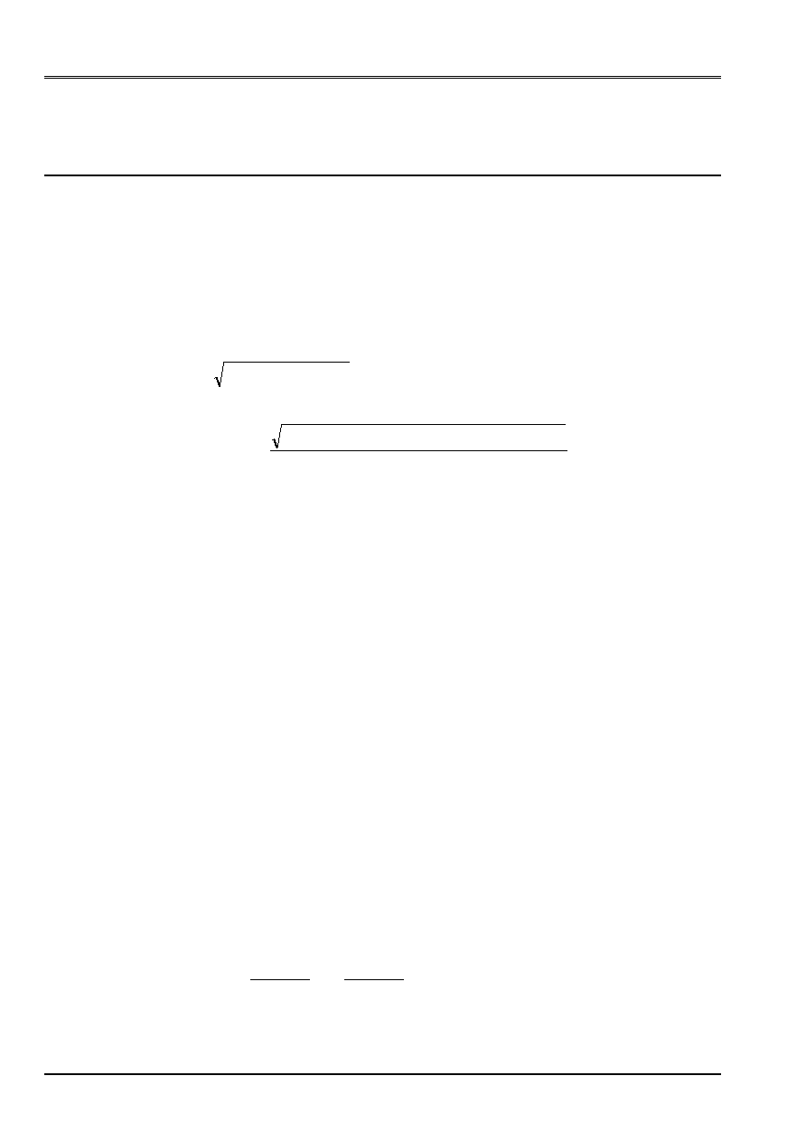
To take into account the retreat of anchoring, the following reasoning is made:
the voltage along the cable is affected by the retreat of anchoring at a distance
D
that one calculates in
solving a problem with two unknown factors: the function
()
F S
*
who represents the force after retreat of
anchoring and the scalar
D
:
[
]
=
-
1
0
E S
F S
F S ds
has
has
D
()
()
*
,
F S
()
is worth
(
)
F E
F
S
0
- -
is the value of the retreat of anchoring
(it is a data)
without retreat of anchoring
Voltage (F)
with passing of anchoring
X-coordinate (S)
D
F S
*
()
, the force after retreat of anchoring, is given starting from the formula [bib1]:
[
]
[
]
F S F S
F D
().
()
()
*
=
2
,
The length
D
will be given in an iterative way thanks to the preceding integral. Other authors
use different relations such as:
[
]
[
]
F S
F D
F D
F S
()
()
()
()
*
-
=
-
For the calculation of
D
, three particular cases can arise:
1) This loss by retreat of anchoring is localized in the area of anchoring. If the cable is
curve, and the sufficiently short length of the cable, it can arrive that
D
that is to say larger than
the length of the cable. In this case, the loss of prestressing due to the retreat of anchoring
apply everywhere. It is necessary to calculate the surface ranging between the two curves
F S
()
and
F S
*
()
, which must be equal to
E S
has
has
, and which thus makes it possible to calculate
F S
*
()
.

Code_Aster
®
Version
7.4
Titrate:
Modeling of the cables of prestressing
Date:
05/04/05
Author (S):
S. MICHEL-PONNELLE, A. ASSIRE
Key
:
R7.01.02-B
Page
:
8/18
Manual of Reference
R7.01 booklet: Modelings for the Civil Engineering and the géomatériaux ones
HT-66/05/002/A
2) If a voltage is applied to each of the two ends of the cable, let us call
)
(
1
S
F
the distribution of initial voltage calculated as if the voltage were applied only to
the first anchoring, and
)
(
2
S
F
the distribution of initial voltage calculated like if the voltage
was applied only to the second anchoring. The value which must be retained in any point of
cable as initial voltage is
(
)
)
(
),
(
)
(
2
1
S
F
S
F
Max
S
F
=
.
3) Lastly, if D is larger than the length of the cable, and when a voltage is
applied to each of the two ends of the cable (superposition of the two preceding cases),
one must apply the following procedure:
- calculation
of
)
(
1
S
F
initial voltage calculated as if the voltage were applied only to
the first anchoring and by taking account of the retreat of anchoring (as in the case
private individual 1),
- calculation
of
)
(
2
S
F
initial voltage calculated as if the voltage were applied only to
the second anchoring and by taking account of the retreat of anchoring (as in the case
private individual 1),
- calculation
of
(
)
)
(
),
(
)
(
2
1
S
F
S
F
Min
S
F
=
.
2.2.3 Deformations differed from steel
The loss by relieving of steel, for an infinite time, is expressed in the following way:
)
(
~
)
(
~
100
5
)
(
0
1000
S
F
S
S
F
J
R
y
has
×
µ
-
×
×
×
(
1000
relieving with 1000 hour in %;
µ
0
the coefficient of relieving of prestressed steel and
y
guaranteed value of the maximum loading to the rupture of the cable).
This relation expresses the loss by relieving of the cables for an infinite time. The BPEL 91 proposes
following formula:
()
R J
J
J
R
m
= +
9
0
.
where
J
indicate the age of the work in days and R
m0
a radius
characteristic obtained by submitting the report/ratio of the section of the structure out of concrete, m ², by
perimeter of the section (in meters) of concrete.
2.2.4 Loss of voltage by instantaneous strains of the concrete
The instantaneous losses are not taken into account in the formula [éq 2.2.1-1] used in
Code_Aster. What the BPEL calls loss of instantaneous voltage is in fact the loss of voltage
induced in cables already posed by the installation of a new group of cables. To modelize it
phenomenon, it is necessary to represent the phasage of setting in prestressed in Aster calculation, i.e.
not to tighten the whole of the cables at the same time but in a successive way by connecting them
CALC_PRECONT
(see test SSNV164).
2.3
Determination of the relations kinematics between steel and concrete
Since the nodes of the mesh of cable do not coincide inevitably with the nodes of the mesh of
concrete, it is necessary to define relations kinematics modelizing perfect adhesion between
cables and concrete.
The following paragraphs describe in the allowing order the space geometrical considerations
to define the concept of vicinity enters the nodes of elements of cable and concrete, then the method of
calculation of the coefficients of the relations kinematics.
Code_Aster
®
Version
7.4
Titrate:
Modeling of the cables of prestressing
Date:
05/04/05
Author (S):
S. MICHEL-PONNELLE, A. ASSIRE
Key
:
R7.01.02-B
Page
:
9/18
Manual of Reference
R7.01 booklet: Modelings for the Civil Engineering and the géomatériaux ones
HT-66/05/002/A
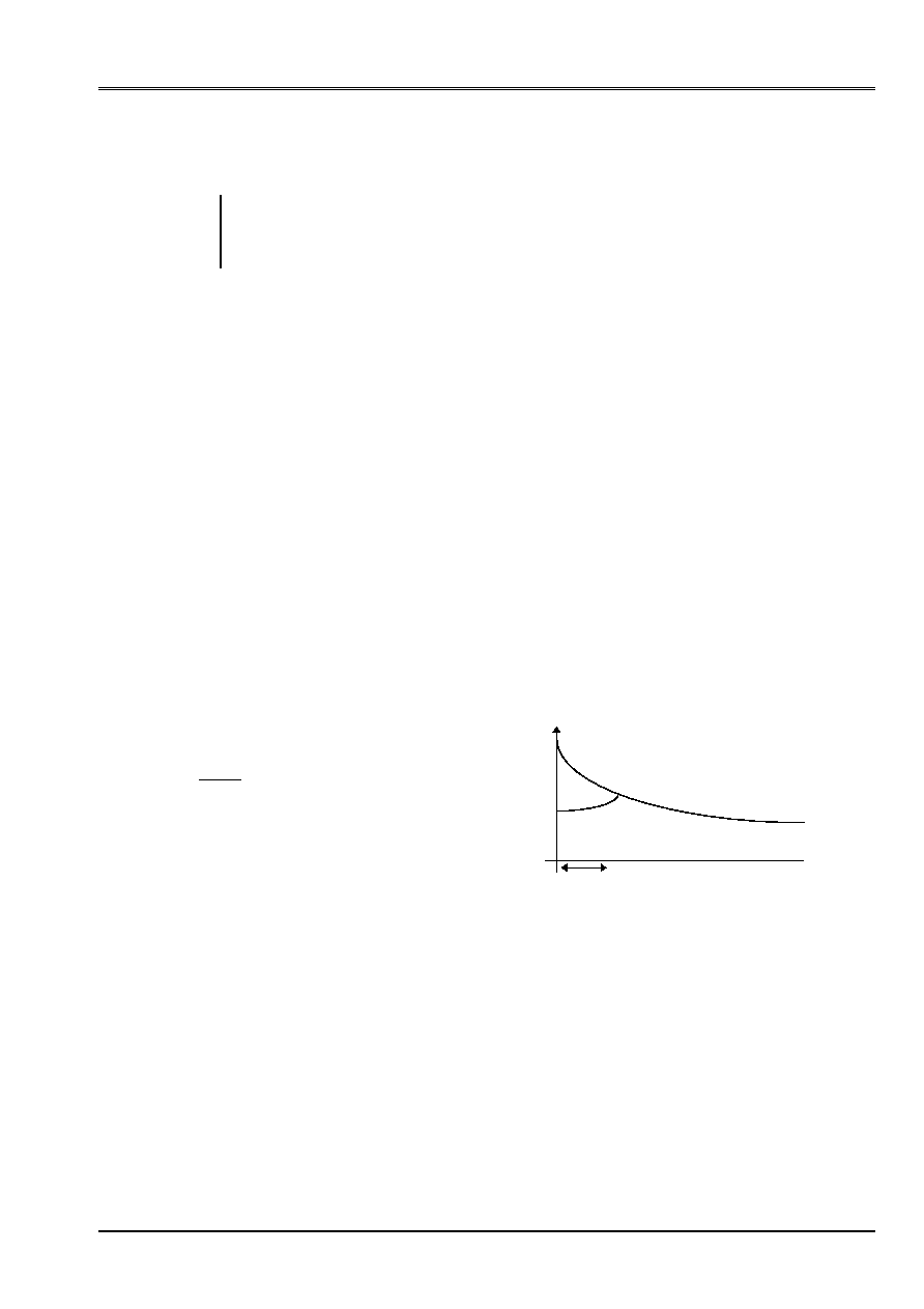
2.3.1 Definition of the close nodes
The calculation of the coefficients of the relations kinematics requires to determine the nodes “close” to
each node of the mesh of the cable. The diagram which follows symbolizes a node cables and a mesh
concrete:
Node cables
Nodes concrete
1
4
3
2
Nodes
neighbors
Element
concrete
The mesh defined by nodes 1, 2, 3, 4 contains the node cables. The close nodes are thus them
nodes 1, 2, 3, 4. If the node cable is located inside an element at p nodes P
1
, P
2
,…, P
N
, then
the nodes P
1
, P
2
,…, P
N
“nodes close” to the node are called cables.
One treats in the same way, the elements of plate without offsetting, and the solid elements.
calculation of the offsetting of each node of the mesh cable is necessary for the calculation of
coefficients of the relations kinematics.
In the case of elements of plate, when the node cable is characterized by a offsetting not no one,
one defines the nodes close as the unit to the nodes node of the element which contains
projection of the node cables in the tangent plan with the mesh concrete. If the node cables (or
well its projection in the tangent plan with the mesh concrete) belongs to a border of an element, it
are the nodes of this border which form the whole of the close nodes.
2.3.2 Calculation of the coefficients of the relations kinematics
In the whole of descriptions which follow the sizes are systematically expressed in
total reference mark of the mesh. The connections kinematics are thus expressed according to the degrees of
freedom expressed in this base. The normals and vectors rotation are expressed in the reference mark
total, except explicit contrary mention.
In modeling finite elements of the structure cable-concrete, the displacement of a material point of
the structure concrete can be expressed easily using the functions of form of the element or of
net concrete whose nodes form the close nodes, according to displacements of the nodes
neighbors of the discretization “concrete”. In the same way, a size or a displacement of a point of the cable,
(or of its projection on the tangent level of the mesh concrete) is identical to the value of this size
at the material structural concrete point which occupies this same position (perfect connection between the concrete
and steel), and is thus expressed according to the value of this same size at the tops of
the element, using the functions of form.
If (X, y, Z) are the co-ordinates of the node cables, or those of its projection, and NR
1
, NR
2
,…, NR
N
functions
forms associated with the nodes concrete P
1
, P
2
,…, P
N
nodes of an element of the mesh concrete (or
nodes of a border of an element of the mesh concrete), and (X
I
, y
I
, Z
I
) co-ordinates of node I, then
the interpolation of a variable U on the element is written:
(
)
(
) (
)
(
)
=
=
=
=
N
I
I
I
N
I
I
I
I
I
U
Z
y
X
NR
Z
y
X
U
Z
y
X
NR
Z
y
X
U
1
1
.
,
,
,
,
.
,
,
,
,
U
being able to be a co-ordinate, or any other nodal data.
Code_Aster
®
Version
7.4
Titrate:
Modeling of the cables of prestressing
Date:
05/04/05
Author (S):
S. MICHEL-PONNELLE, A. ASSIRE
Key
:
R7.01.02-B
Page
:
10/18
Manual of Reference
R7.01 booklet: Modelings for the Civil Engineering and the géomatériaux ones
HT-66/05/002/A
The connections kinematics make it possible to express the identity of displacement between the node of the mesh
cable, and the material point concrete which occupies the same position. This corresponds to the assumption of one
perfect connection between the concrete and the cable.
2.3.2.1 Case where the concrete is modelized by massive finite elements
By taking again the preceding notations and while considering
C
C
C
dz
Dy
dx
,
,
displacements of the node
cable, and
dx Dy dz
jb
jb
jb
,
,
displacements of the nodes J (J = 1, N) of the structure concrete neighbors of the node
cable we obtain the following relations:
=
=
=
=
=
=
N
I
B
I
C
C
C
I
C
N
I
B
I
C
C
C
I
C
N
I
B
I
C
C
C
I
C
dz
Z
y
X
NR
dz
Dy
Z
y
X
NR
Dy
dx
Z
y
X
NR
dx
1
1
1
)
,
,
(
)
,
,
(
)
,
,
(
N being the number of nodes of the element concrete neighbors of the node of the cable, or that of one of its
borders. For each node of the cable one obtains 3 relations kinematics between displacements
nodes of the two mesh cables and concrete.
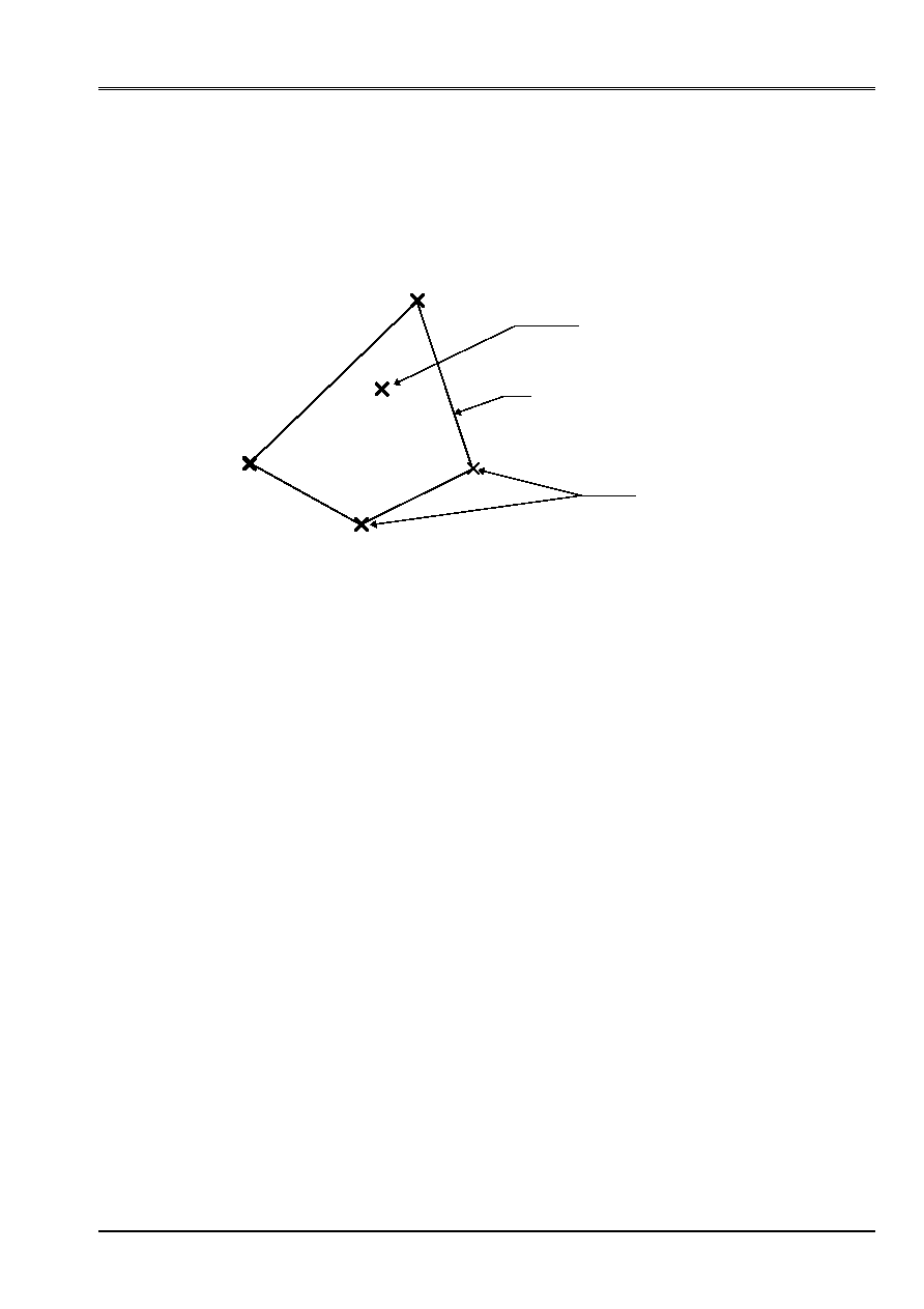
2.3.2.2 Case where the concrete is modelized by finite elements of plate
P
2
P
1
P
B
3
P
C
P
N
That is to say
C
P
0
the initial position of a point of cable in the not deformed geometry and is
C
P
the position
this same point after deformation. Let us call
p
P
0
the projection of
C
P
0
on the surface of the layer
means of the concrete hull not deformed and
p
P
the projection of
C
P
on the surface of the average layer
concrete hull deformed. That is to say
0
N
the normal in the average plan of the concrete hull in
p
P
0
and
N
that in
p
P
.
p
O
P
is given by:
-
-
-
-
=
Z
y
X
Z
y
X
B
C
B
C
B
C
C
C
C
p
p
p
N
N
N
N
N
N
Z
Z
y
y
X
X
Z
y
X
Z
y
X
0
0
0
0
0
0
0
0
0
0
0
0
0
0
0
0
0
0
.
.
p
P
is given by:
-
-
-
-
=
Z
y
X
Z
y
X
B
C
B
C
B
C
C
C
C
p
p
p
N
N
N
N
N
N
Z
Z
y
y
X
X
Z
y
X
Z
y
X
.
.
Code_Aster
®
Version
7.4
Titrate:
Modeling of the cables of prestressing
Date:
05/04/05
Author (S):
S. MICHEL-PONNELLE, A. ASSIRE
Key
:
R7.01.02-B
Page
:
11/18
Manual of Reference
R7.01 booklet: Modelings for the Civil Engineering and the géomatériaux ones
HT-66/05/002/A
The point
p
O
P
belongs to a mesh of concrete plate whose nodes are noted
P P
P
B
B
B
1
2
3
,
and
.
One defines the offsetting of the cable compared to the concrete hull as the distance
C
p
P
P
E
0
0
=
and
the assumption is made that this offsetting does not vary when the structure becomes deformed
:
C
p
C
p
P
P
P
P
E
=
=
0
0
One introduces displacements of the points of the cable and his projection:
=
C
C
C
C
C
dz
Dy
dx
P
P
0
=
=
=
=
=
=
=
N
I
B
I
p
p
p
I
p
N
I
B
I
p
p
p
I
p
N
I
B
I
p
p
p
I
p
p
p
dz
Z
y
X
NR
dz
Dy
Z
y
X
NR
Dy
dx
Z
y
X
NR
dx
P
P
1
0
0
0
1
0
0
0
1
0
0
0
0
)
,
,
(
)
,
,
(
)
,
,
(
One introduces the vector “rotation”
plate at the point
p
P
and degrees of freedom of rotation of
nodes of the plate:
=
=
=
=
=
=
=
N
I
B
I
p
p
p
I
B
N
I
B
I
p
p
p
I
B
N
I
B
I
p
p
p
I
B
drz
Z
y
X
NR
drz
dry
Z
y
X
NR
dry
drx
Z
y
X
NR
drx
1
0
0
0
1
0
0
0
1
0
0
0
)
,
,
(
)
,
,
(
)
,
,
(
By definition of
, one a:
0
0
N
N
N
v
R
v
v
=
-
One can then write:
N
E
P
P
N
E
P
P
C
p
C
p
=
=
0
0
0
By withdrawing these two equations, by taking account of the definition of
one finds:
(
)
(
)
(
)
-
=
-
-
=
-
-
=
-
X
p
y
p
p
C
Z
p
X
p
p
C
y
p
Z
p
p
C
N
dry
N
drx
E
dz
dz
N
drx
N
drz
E
Dy
Dy
N
drz
N
dry
E
dx
dx
0
0
0
0
0
0
.
.
.
.
.
.
.
.
.
By injecting into this last equation the functions of form, one has finally:
(
)
(
)
(
)
(
)
(
)
(
)
(
)
(
)
(
)
-
=
-
-
=
-
-
=
-
=
=
=
=
=
=
=
=
=
X
N
I
B
I
p
p
p
I
y
N
I
B
I
p
p
p
I
N
I
B
I
p
p
p
I
C
Z
N
I
B
I
p
p
p
I
X
N
I
B
I
p
p
p
I
N
I
B
I
p
p
p
I
C
y
N
I
B
I
p
p
p
I
Z
N
I
B
I
p
p
p
I
N
I
B
I
p
p
p
I
C
N
dry
Z
y
X
NR
N
drx
Z
y
X
NR
E
dz
Z
y
X
NR
dz
N
drx
Z
y
X
NR
N
drz
Z
y
X
NR
E
Dy
Z
y
X
NR
Dy
N
drz
Z
y
X
NR
N
dry
Z
y
X
NR
E
dx
Z
y
X
NR
dx
0
1
0
1
1
0
1
0
1
1
0
1
0
1
1
.
,
,
.
,
,
.
,
,
.
,
,
.
,
,
.
,
,
.
,
,
.
,
,
.
,
,
Code_Aster
®
Version
7.4
Titrate:
Modeling of the cables of prestressing
Date:
05/04/05
Author (S):
S. MICHEL-PONNELLE, A. ASSIRE
Key
:
R7.01.02-B
Page
:
12/18
Manual of Reference
R7.01 booklet: Modelings for the Civil Engineering and the géomatériaux ones
HT-66/05/002/A
2.3.2.3 Case where the node of the cable is projected on a node of the mesh concrete
The distance enters projection
p
P
0
node cables
C
P
0
and a node concrete
B
I
P
is given by:
D
P P
X
X
y
y
Z
Z
X
X
y
y
Z
Z
N
N
P ib
C
ib
C
ib
C
ib
C
ib
C
ib
C
ib
=
=
-
-
-
-
-
-
-
0
0
0
.
.
R
R
If it happens that this distance is null (in practice lower than 10
- 5
), it is that the node cables
project at the top of a concrete mesh, and then the relations kinematics are simplified:
(
)
(
)
(
)
-
=
-
-
=
-
-
=
-
X
p
I
y
p
I
p
I
C
Z
p
I
X
p
I
p
I
C
y
p
I
Z
p
I
p
I
C
N
dry
N
drx
E
dz
dz
N
drx
N
drz
E
Dy
Dy
N
drz
N
dry
E
dx
dx
0
0
0
0
0
0
.
.
.
.
.
.
.
.
.
These relations are the general relations in which:
0
)
,
,
(
=
p
p
p
J
Z
y
X
NR
if
J I
.
2.4
Processing of the areas of end of the cable
The modeling of a cable of prestressed such as it is made in Code_Aster consists with
to represent the unit cables, sheath of passage, and all the parts of anchoring, only thanks to
a succession of elements of bar. The link between the elements of cables and the concrete medium is ensured by
conditions kinematics on DDLs of each node of the cable, and those of the elements
concrete crossed.
When the setting in voltage of the cable is applied, it is observed that the reactions generated with
ends of the cables on the concrete create levels of stresses much higher than reality, and
cause the damage of the concrete. As example, in certain studies, one could observe
compressive stresses of more than 200 MPa, which largely exceeds the value
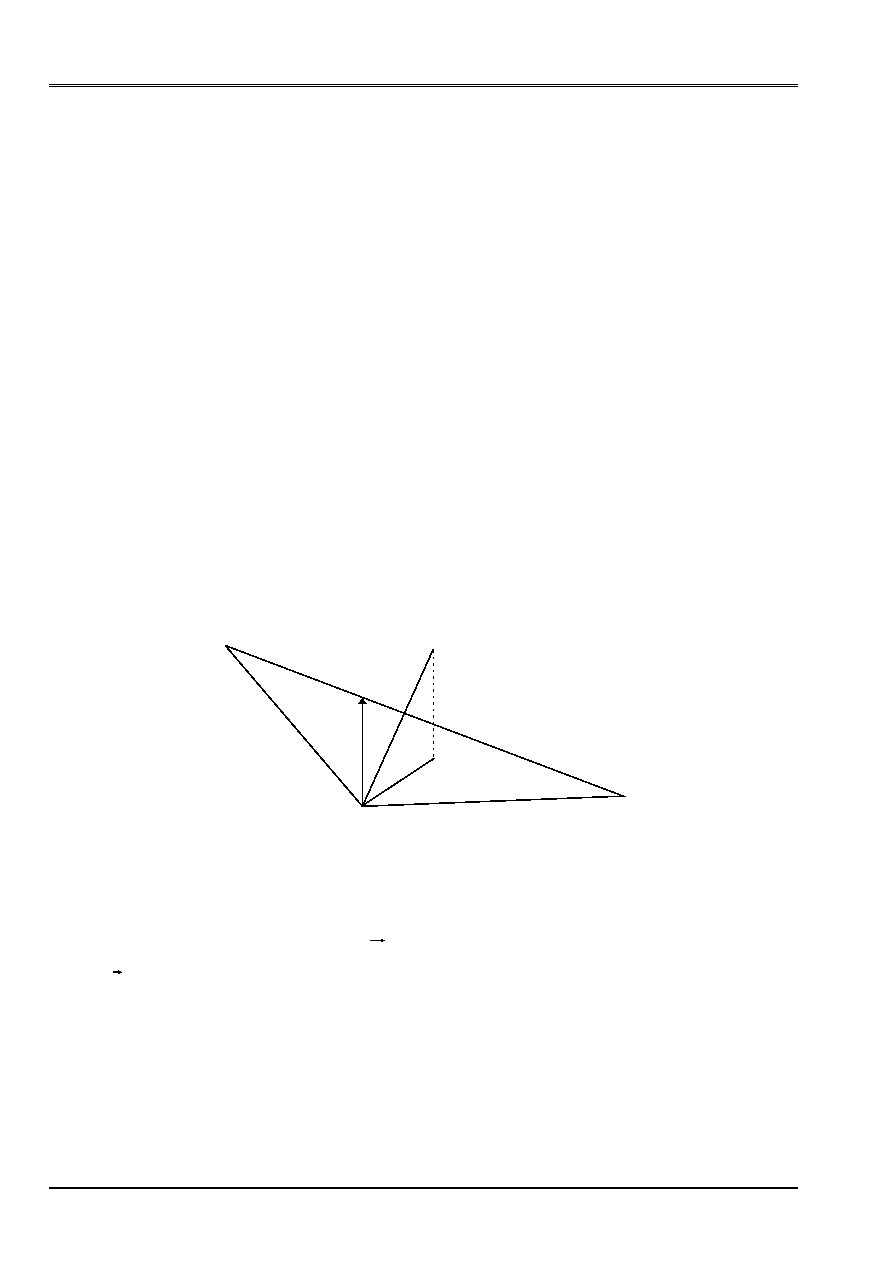
experimental observed (40 MPa). In reality, this phenomenon is not observed thanks to the setting
in place of a cone of diffusion of stress (see drawing below) which distributes the force of
prestressed on a great surface of the concrete. In the case of model EFF this surface does not exist,
since the force is directly taken again by a node.
With
Real situation
Model EFF without cone
This way of modeling has several disadvantages:
·
the concentration of this effort crushes the concrete,
·
the space discretization of the model changes the results.
Code_Aster
®
Version
7.4
Titrate:
Modeling of the cables of prestressing
Date:
05/04/05
Author (S):
S. MICHEL-PONNELLE, A. ASSIRE
Key
:
R7.01.02-B
Page
:
13/18
Manual of Reference
R7.01 booklet: Modelings for the Civil Engineering and the géomatériaux ones
HT-66/05/002/A
To cure this problem, the key word
CONE
of the operator
DEFI_CABLE_BP
allows to distribute
this force of prestressed either on a node, but on all the nodes contained in a volume
(all the nodes of this volume are dependant between them to form a rigid solid) delimited by a cylinder
of radius R and length L, representing the equivalent of the area of influence of the cone
of blooming of an anchoring (see figure below).
length
radius
The identification and the creation of the relations kinematics between the nodes of the concrete and the cable are done
in an automatic way by the control
DEFI_CABLE_BP
, where the new data R and L will be with
to provide by the user.
2.5 Note: calculation of the voltage of the cable as a loading
mechanics
We made the choice leave the elements of cable in the mechanical model support of calculation
by finite elements (linear or not). So there is no calculation of equivalent force to defer to
nodes of the mesh. One is simply satisfied to say that the cables of prestressing have a state of
initial stress not no one. This state of stress is that deduced from the voltage as calculated by
DEFI_CABLE_BP
.
For reasons of simplicity, the data-processing object created by the operator
DEFI_CABLE_BP
is a table
memorizing values with the nodes of the cable. Then let us consider two related elements of the cable:
e1 of N1 nodes and N2, and
e2 of node N2 and N3.
We suppose that
L
1
and
S
1
are the length and the section of an element e1 and that
L
2
and
S
2
are
length and the section of the element e2.
N2
e1
e2
N3
N1
DEFI_CABLE_BP
with the node N2 a voltage will calculate
T
NR
2
defined by:
+
=
2
1
2
1
2
)
(
)
(
2
1
L
ds
S
T
L
ds
S
T
T
E
E
NR
Code_Aster
®
Version
7.4
Titrate:
Modeling of the cables of prestressing
Date:
05/04/05
Author (S):
S. MICHEL-PONNELLE, A. ASSIRE
Key
:
R7.01.02-B
Page
:
14/18
Manual of Reference
R7.01 booklet: Modelings for the Civil Engineering and the géomatériaux ones
HT-66/05/002/A
Conversely, for calculation finite element, the operator
STAT_NON_LINE
will consider that the stress
initial in the element e1 is
0
1
1
1
2
2
E
NR
NR
T
T
S
=
+
Note:
It will be always considered that the law of behavior of the cable is of incremental type.
3
macro-control
CALC_PRECONT
3.1
Why a macro-control for the setting in voltage?
It is possible to transform the voltage in the cables calculated by
DEFI_CABLE_BP
in one
loading directly taken into account by
STAT_NON_LINE
thanks to the control
AFFE_CHAR_MECA
operand
RELA_CINE_BP (SIGM_BPEL=' OUI')
. In this case, the voltage is taken
in account like an initial state of stress at the time of the resolution of complete problem EFF.
F
0
F
0
Initially
F
F
With balance
The resolution of the problem makes it possible to reach a state of balance between the cable of prestressed and it
remain structure after instantaneous strain. Indeed, under the action of the voltage of the cable,
the unit cables (S) and concrete will be compressed compared to the initial position (cable in voltage,
mesh not deformed). The length of the cable thus will decrease, and the initial voltage also goes, by
consequence sees, to decrease. One thus obtains a final state with a voltage in the cable different
voltage calculated initially. It is then essential to increase proportionally
voltage applied in situ to the level them anchorings to take account of this loss.
The use of the macro-control
CALC_PRECONT
allows to avoid this phase of correction, in
obtaining the state of balance of the structure with a voltage in the cables equalizes with the voltage
lawful. In addition because of adopted method, it allows in addition to applying the voltage in
several pitches of time, which can be interesting in the event of plasticization or of damage of
concrete. It makes it possible moreover to tighten the cables in a nonsimultaneous way and thus of manner more
near to the reality of the building sites.
To profit from these advantages, the loading is applied in the form of an external loading
and not like an initial state, which allows the progressive loading of the structure. In addition, for
to avoid the loss of voltage in the cable, the idea is not to make act the rigidity of the cables during
phase of setting in voltage (cf [bib3]).
The various stages carried out by the macro-control are here detailed.
Code_Aster
®
Version
7.4
Titrate:
Modeling of the cables of prestressing
Date:
05/04/05
Author (S):
S. MICHEL-PONNELLE, A. ASSIRE
Key
:
R7.01.02-B
Page
:
15/18
Manual of Reference
R7.01 booklet: Modelings for the Civil Engineering and the géomatériaux ones
HT-66/05/002/A
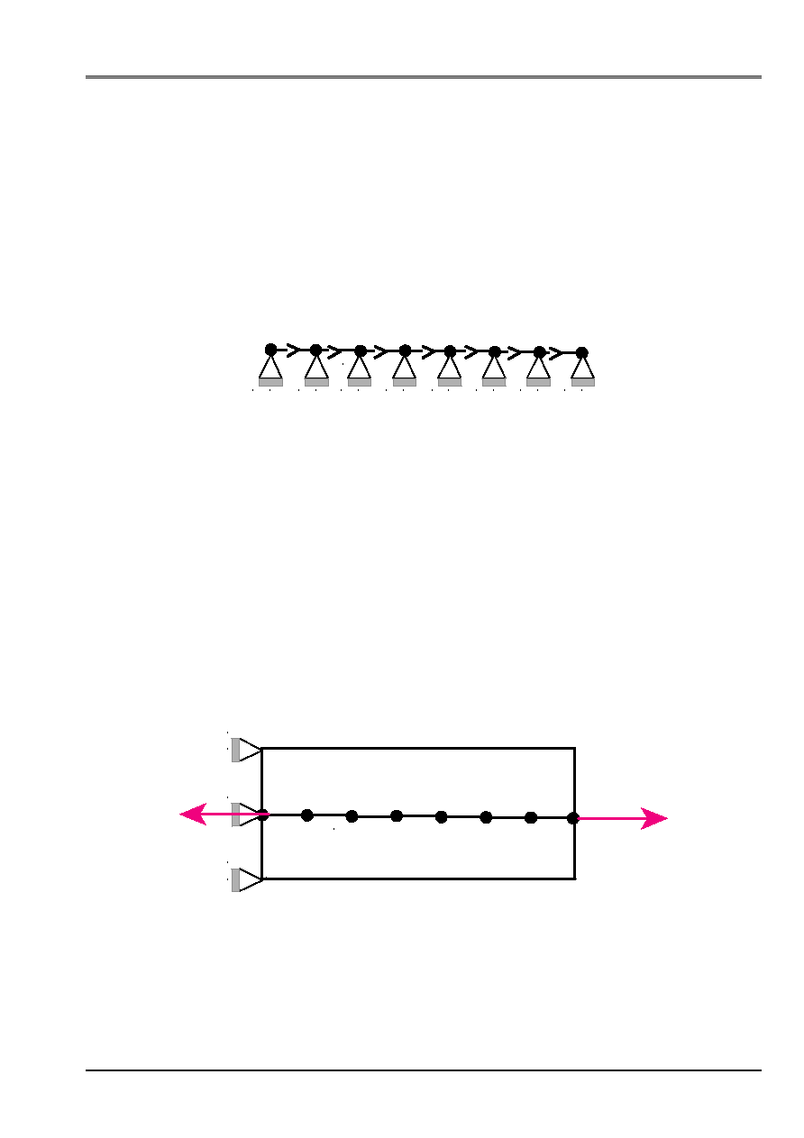
3.1.1 Stage 1: calculation of the equivalent nodal forces
This stage consists in transforming the internal voltages of the cables calculated by
DEFI_CABLE_BP
in
an external loading. For that, one carries out a first
STAT_NON_LINE
only on the cables
that one wishes to put in prestressing, with the following loading:
·
cable embedded
·
the voltage given by
DEFI_CABLE_BP
T
T
T
Appear 3.1.1-a: Loading at stage 1
One calculates the nodal efforts on the cable. One recovers these efforts thanks to
CREA_CHAMP
. And one
built the vector associated loading
F
.
3.1.2 Stage 2: application of prestressed to the concrete
The following stage consists in applying prestressing to the concrete structure, without making take part
rigidity of the cable. For that, one supposes for this calculation that the Young modulus of steel is null. One
can choose to apply the loading of prestressed in only one pitch of time or several pitches
time if the concrete is damaged.
The loading is thus the following:
·
blocking of the rigid movements of body for the concrete,
·
nodal efforts resulting from the first calculation on the cable,
·
the connections kinematics between the cable and the concrete.
F
Ecable = 0
Appear 3.1.2-a: Loading at stage 2
Code_Aster
®
Version
7.4
Titrate:
Modeling of the cables of prestressing
Date:
05/04/05
Author (S):
S. MICHEL-PONNELLE, A. ASSIRE
Key
:
R7.01.02-B
Page
:
16/18
Manual of Reference
R7.01 booklet: Modelings for the Civil Engineering and the géomatériaux ones
HT-66/05/002/A
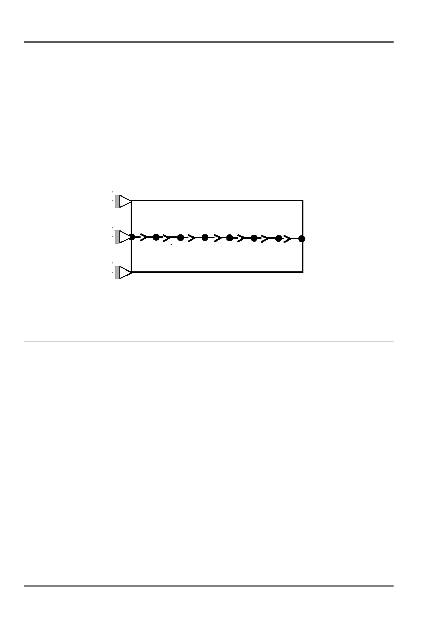
3.1.3 Stage 3: tilting of the external efforts in interior efforts
Before continuing calculation in a traditional way, it is necessary of retransformer the efforts
outsides which made it possible to deform the concrete structure in interior efforts. This operation is done
without amendment on displacements and the stresses of the whole of the structure, since
balance was reached at stage 2: it is about a simple artifice to be able to continue calculation.
loading is thus the following:
·
blocking of the rigid movements of body for the concrete,
·
the connections kinematics between the cable and the concrete,
·
voltage in the cables.
T
T
T
Appear 3.1.3-a: Loading at stage 3
4
Procedure of modeling
4.1
Various stages: standard case
To manage to modelize a concrete structure prestresses the procedure to be followed is as follows:
·
to modelize the concrete elements (
DKT
,
2D
or
3D
),
·
to modelize the cables of prestressed by elements bars with two nodes (
BAR
),
·
to allot to the elements bars the mechanical characteristics of the cables of prestressing,
·
thanks to the operator
DEFI_CABLE_BP
to calculate the data kinematics (relations
kinematics between the nodes of the cable and those of the concrete elements) and statics (profile of
voltage along the cables),
·
to define the data kinematics like mechanical loading,
·
to call upon the operator
CALC_PRECONT
,
·
to solve the problem with the operator
STAT_NON_LINE
by integrating only them
data kinematics and loadings other than prestressing.
For more practical information, to refer to the document [U2.03.06].
4.2
Particular case: DKT
For the moment, the macro-control
CALC_PRECONT
do not function if the elements concrete are
of type DKT. In this case, it is advisable to adopt the following procedure:
·
to modelize the concrete elements (
DKT
),
·
to modelize the cables of prestressed by elements bars with two nodes (
BAR
),

Code_Aster
®
Version
7.4
Titrate:
Modeling of the cables of prestressing
Date:
05/04/05
Author (S):
S. MICHEL-PONNELLE, A. ASSIRE
Key
:
R7.01.02-B
Page
:
17/18
Manual of Reference
R7.01 booklet: Modelings for the Civil Engineering and the géomatériaux ones
HT-66/05/002/A
·
to allot to the elements bars the mechanical characteristics of the cables of prestressing,
·
thanks to the operator
DEFI_CABLE_BP
to calculate the data kinematics (relations
kinematics between the nodes of the cable and those of the concrete elements) and statics (profile of
voltage along the cables),
·
to apply these data kinematics and statics like a mechanical loading,
·
to solve problem with the operator
STAT_NON_LINE
by integrating all the loadings.
For the exit of this calculation it is necessary to determine the coefficients of correction to apply to the initial voltages
applied to the cables (on the level of the statement of the operator
DEFI_CABLE_BP
) allowing
to compensate for the loss by instantaneous strain of the structure.
Once the command file modified by these coefficients of correction, the modeling of the cables
of prestressing is accomplished.
Attention, in the case of sequence of
STAT_NON_LINE
, it is appropriate starting from the second call, of
to include in the loading only the relations kinematics and not the voltage in the cables, under
pains to add this voltage, with each calculation.
4.3
Precautions of use and remarks
It is recommended to limit the recourse to a great number of relations kinematics under sorrow
to weigh down the calculating time. However, when a node of the elements of bar constituting the cables
coincide topologically with a node concrete, it does not have there a kinematic addition of relation.
If a first is carried out
STAT_NON_LINE
before putting in voltage in the cables, it is
preferable to decontaminate the cables, either by not taking them into account in the model, or in their
affecting a voltage constantly null (law of behavior
WITHOUT
), and while including in
loading the relations kinematics binding the cable to the concrete.
If one carries out a phasage setting in prestressing, it is necessary to think of including them
relations kinematics in the loading for the cables already tended at the preceding stages.

Code_Aster
®
Version
7.4
Titrate:
Modeling of the cables of prestressing
Date:
05/04/05
Author (S):
S. MICHEL-PONNELLE, A. ASSIRE
Key
:
R7.01.02-B
Page
:
18/18
Manual of Reference
R7.01 booklet: Modelings for the Civil Engineering and the géomatériaux ones
HT-66/05/002/A
5 Bibliography
[1]
Rules BPEL 91, technical Rules of design and calculation of the works and constructions
out of prestressed concrete following the method of the limiting states. CSTB, ISBN 2-86891-214-1.
[2]
P. MASSIN: “Elements of plate DKR, DST, DKQ, DSQ and Manual Q4Eg” of Reference
Aster [R3.07.03].
[3]
S. GHAVAMIAN, E. LORENTZ: Improvement of the functionalities of the taking into account of
prestressed in Code_Aster, CR AMA 2002-01