Modeling of the contact

Code_Aster

Version

6.4

Titrate:

Modeling of the contact

Date

04/11/03

Author (S):

S. LAMARCHE

Key

U2.04.04-A

Page

1/28

Instruction manual

U2.04 booklet: Nonlinear mechanics

HT-66/03/002/A

Organization (S):

EDF-R & D/AMA

Instruction manual
U2.04 booklet: Nonlinear mechanics
Document: U2.04.04

Modeling of the contact

Summary:

One describes in this document the methods available in Code_Aster to deal with the problems of contact
with or without friction, into small or great displacements.
One will treat in details the loads of contact, used by the operators

STAT_NON_LINE

and

DYNA_NON_LINE

. And one will approach the modeling of the specific contact on

DYNA_TRAN_MODAL

or with

elements

DIS_CONTACT

Code_Aster

Version

6.4

Titrate:

Modeling of the contact

Date

04/11/03

Author (S):

S. LAMARCHE

Key

U2.04.04-A

Page

4/28

Instruction manual

U2.04 booklet: Nonlinear mechanics

HT-66/03/002/A

1 Introduction

One speaks about study of contact as soon as there can be interaction of contact during calculation.
It is possible to modelize the problems of contact-impact and contact-friction with
Code_Aster, into small or great displacements.
This document reviews the various methods available, underlines the encountered difficulties
and gives consultings of use. One will privilege the processing of the contact by the loads of contact. It
exist other methods, they relate to only the specific contact and they are presented in
chapter 6.

General step

The contact is declared in

AFFE_CHAR_MECA

, like a load. All conditions of contact

must be declared in the same one

AFFE_CHAR_MECA

(each one in an occurrence of the key word

CONTACT

Initially, one indicates surfaces between which one wants to treat the contact.
One then chooses to treat the contact with or without friction. In the case of the contact with
friction, it is necessary to give the coefficient of friction.
One also indicates the methods of calculation to be used and the method of pairing.
It is through these stages that one defines all the parameters of the contact.
They take place in the operator

AFFE_CHAR_MECA

The conditions of contact are thus declared like a load. They are used like such
(key word

EXCIT

) in the operators mechanics

STAT_NON_LINE

DYNA_NON_LINE

Once completed calculation, one can make a postprocessing of the efforts of contact.

Useful readings

Documentation here presents has the role to guide the user at the time of a modeling in contact
friction. It takes again the essential indications and gives consultings of use.
It does not replace the reading of U4 documentations of each operator. The user will find
in these documentations the syntax of the operator, as well as the significance of each parameter.
In addition, the user who wishes to have more detailed approach and comments on
algorithms or the equations of the contact, will refer to the reference materials R5: [R5.03.50]
and [R5.03.51].
Examples are provided here to illustrate certain points. One will be able in addition to refer to the cases
test (V6 documentation) and to be inspired some.

Plan

In a second part, we will give some elementary definitions specific to
modeling of the contact.
Partly 3, one finds a short description of the Code_Aster operators concerned.
In parts 4 and 5, one will approach the difficulties of modeling and calculation. One will find in
these parts consultings to use the contact in Code_Aster.
Part 6 is devoted to other modelings of the contact in Code_Aster. It is reserved for
specific contact.

Code_Aster

Version

6.4

Titrate:

Modeling of the contact

Date

04/11/03

Author (S):

S. LAMARCHE

Key

U2.04.04-A

Page

5/28

Instruction manual

U2.04 booklet: Nonlinear mechanics

HT-66/03/002/A

2 Definitions

Contact

The taking into account of the contact by Code_Aster does not go from oneself. Without specific statement, two
elements can occupy the same place of space.
If it is provided that two surfaces can come into contact during calculation, one should be done
statement of contact. Surfaces in questions are called surfaces of contact.

The surface of contact is 2D for a structure 3D, 1D for a structure 2D.

Master/Slave

When it is declared that two surfaces S1 and S2 are likely to come into contact, Code_Aster writes them
suitable relations. These relations are not symmetrical. This is why one is brought to
to distinguish two surfaces, to the first one gives the name of Master, at the second the name of slave.
The processing of the contact consists in preventing the nodes slaves from penetrating surface Master.

Note:

For the methods

LAGRANGE

and

STRESS

, Code_Aster treats the contact while applying

multipliers of Lagrange carried by the nodes slaves.

One understands in this case that the main choice of surface and surface slave can have one
influence on the result of calculation. One will find thereafter consultings to make this choice.

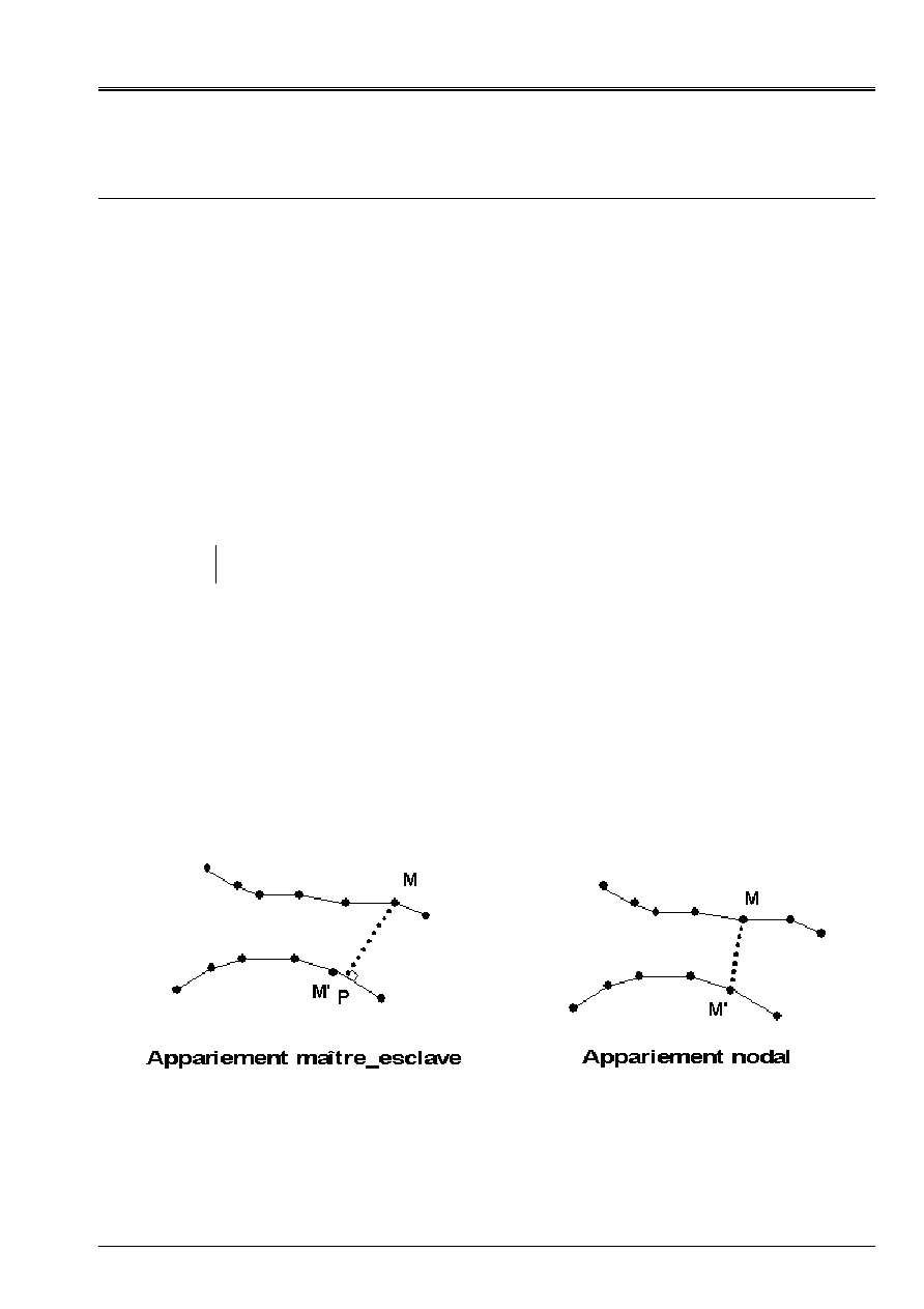
Pairing

Pairing is the phase of calculation where Code_Aster calculates between which point slave and which point
Master (or which mesh Master) will be written the relations of contact.
Pairing is called

“NODAL”

pairing enters a node slave and a main node.

Pairing is called

“MASTER-SLAVE”

pairing enters a node slave and its projection

on surface Master.

Appear 2-a: Pairing

“MASTER-SLAVE”

and pairing

“NODAL”

Code_Aster

Version

6.4

Titrate:

Modeling of the contact

Date

04/11/03

Author (S):

S. LAMARCHE

Key

U2.04.04-A

Page

6/28

Instruction manual

U2.04 booklet: Nonlinear mechanics

HT-66/03/002/A

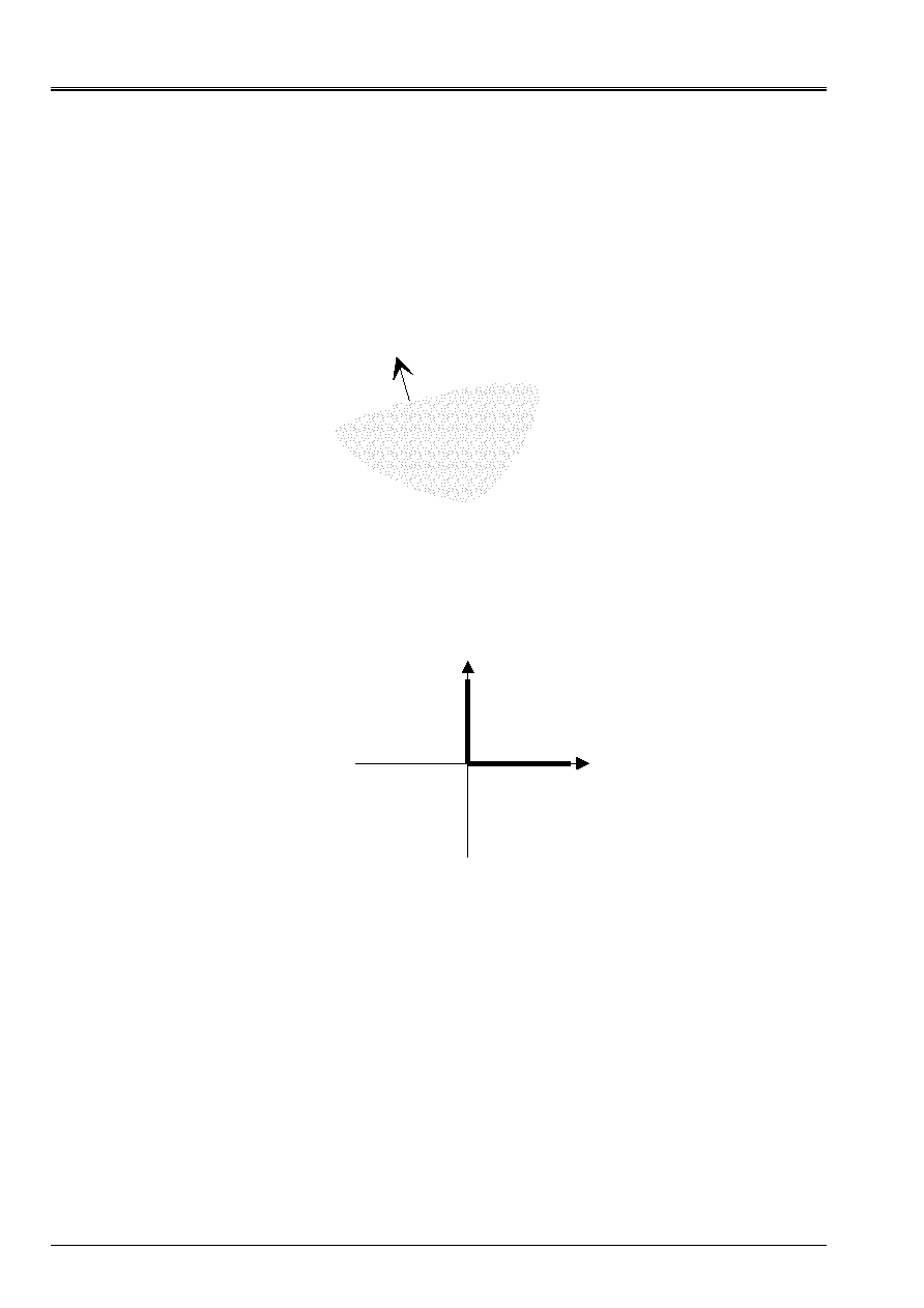
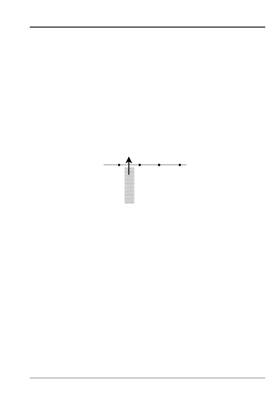
Normal

The normals on the surfaces have a very important role at the time of pairing and writing of
relation of the contact.
Their direction allows the projection of the points slaves on surfaces Master, but they are too
used for the writing of the equations of contact. Their direction makes it possible to distinguish the interior of
the outside of the structure. The normals must always be outgoing.
This is why it is essential always to define and correctly direct the normals of
surfaces in contact.

Appear 2-b: the normal must be outgoing

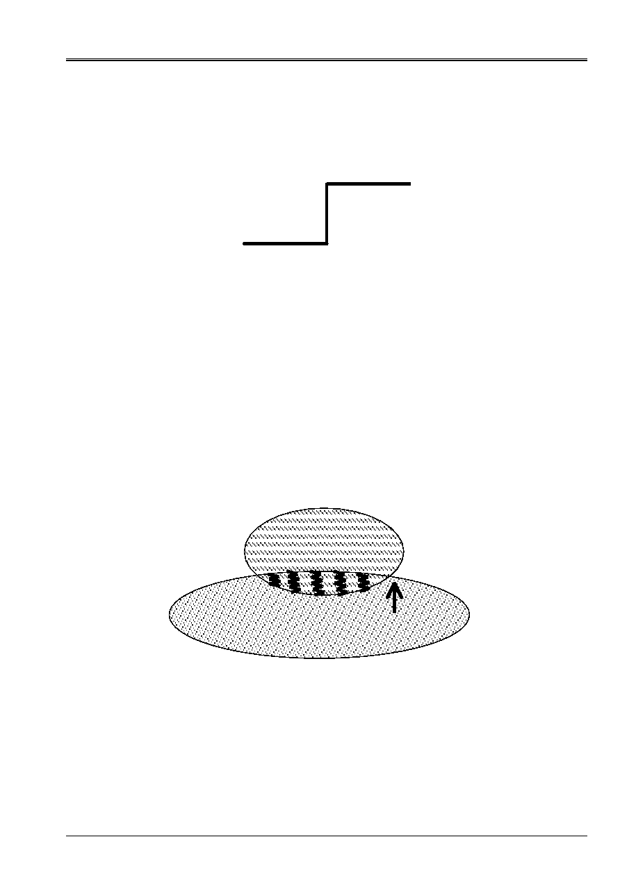
Conditions of Signorini

The conditions of Signorini are the conditions of noninterpenetration.

Appear 1-c: Condition of Signorini

They say that the normal force of contact is null when there is not contact (DNN > 0), and that
interpenetration (i.e. DNN

0) are impossible. If there is contact, normal reaction

can take any positive value (effort of repulsion) which answers the mechanical problem
and which prevents the interpenetration.

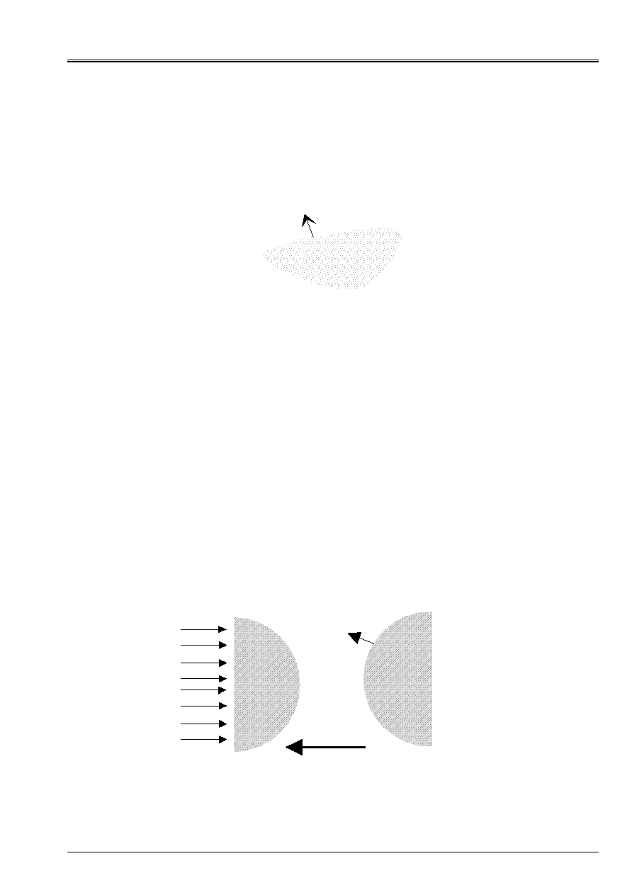
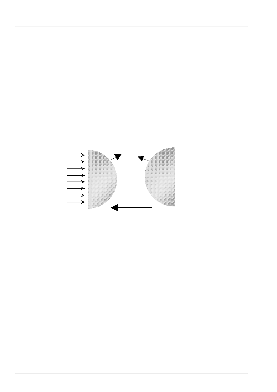
Force contact

During the contact, two surfaces in contact generate forces one on the other. These forces
allow two surfaces not to interpenetrate. They respect the principle of action and
reaction. One has access to these forces during postprocessing.
These forces are always forces of repulsion (to move away surfaces in contact).
They do not act remotely, i.e. they are null when two surfaces
do not touch.

Force
normal

DNN

Code_Aster

Version

6.4

Titrate:

Modeling of the contact

Date

04/11/03

Author (S):

S. LAMARCHE

Key

U2.04.04-A

Page

7/28

Instruction manual

U2.04 booklet: Nonlinear mechanics

HT-66/03/002/A

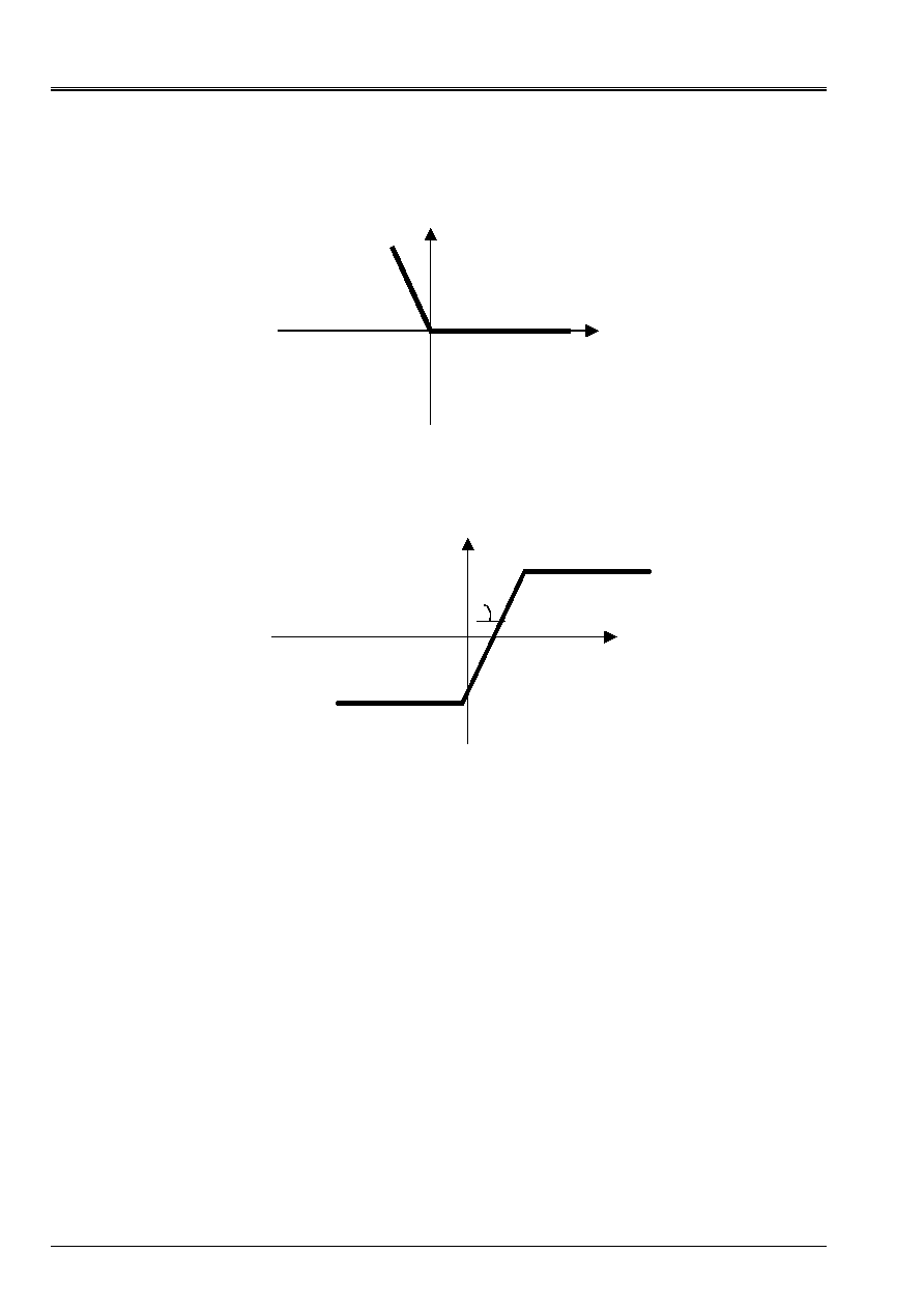
Coefficient of friction µ

Friction is taken into account by the law of Coulomb.

Appear 2D: Law of Coulomb

This law utilizes a coefficient µ, called coefficient of Coulomb. During the phase of adherence,
the point does not move (null speed). During the phase of slip, the point has a speed not
null, it is subjected to a tangent reaction equalizes with µ time the normal reaction.
The coefficient of Coulomb depends on surfaces in contact.
If the coefficient of friction is null (i.e., if there is no friction), there is no reaction
tangential.

Penalization

One can treat the contact in a penalized way.

For the normal direction, in other words, once in contact, the structure are pushed back by
a stiffness. This stiffness exerts a repulsive effort between the structures. During this phase, there is
interpenetration of the structures.
One fixes this stiffness with the normal coefficient of penalization

E_N

Appear 2nd: Coefficient of normal penalization

Code_Aster

Version

6.4

Titrate:

Modeling of the contact

Date

04/11/03

Author (S):

S. LAMARCHE

Key

U2.04.04-A

Page

8/28

Instruction manual

U2.04 booklet: Nonlinear mechanics

HT-66/03/002/A

This penalization corresponds to a regularization of the curve of Signorini:

Appear 2-f: Condition of Signorini penalized

For friction, the penalization appears on the curve of Coulomb.
In this case, there is no phase of adherence, the infinite slope is replaced by a slope finished of
value the tangent coefficient of penalization

E_T

Appear 2-g: Law of Coulomb penalized

One should not confuse the tangent coefficient of penalization

E_T

with the coefficient of friction µ.

On the preceding curve, the first fixes the slope at the origin, the second fixes the value of the bearing.

Loads of contact

In Code_Aster, one speaks about loads of contact. All the statements of the contact are done like
a statement of load. One defines the parameters in

AFFE_CHAR_MECA

and one uses them in

key word

EXCIT

of the operator of calculation.

Interpenetration

One speaks about interpenetration when a structure penetrates inside the other and reciprocally.
The interpenetration is not a physical phenomenon. A physical object can come to be crushed on one
other but does not penetrate in the matter of the other.

Force normal

DNN

F = -

E_N

.dn

µ.|R

- µ.|R

- v

E_T

Code_Aster

Version

6.4

Titrate:

Modeling of the contact

Date

04/11/03

Author (S):

S. LAMARCHE

Key

U2.04.04-A

Page

9/28

Instruction manual

U2.04 booklet: Nonlinear mechanics

HT-66/03/002/A

Exact solution

One will use the expression “solution exact” to indicate a solution which follows the laws exactly of
contact (conditions of Signorini and law of Coulomb).
In particular, an exact solution does not allow the interpenetration.
The exact solution is obtained without the recourse to coefficients of penalization chosen by
the user, and on which strongly the solution depends.
Obviously, an “exact” solution is not inevitably physically acceptable, and it depends
always other parameters of calculation and modeling.

Specific contact

One speaks about specific contact when two “surfaces” potentially in contact are reduced to
points. For example, on telegraphic models, one can be brought to use the specific contact.

One can use the specific contact in 2D or 3D.
It should not be confused with nodal pairing where the relations are written between two nodes but
where the contact can be done between two surfaces (or segments), and pairings can evolve/move with
run of calculation.
One can treat the specific contact with the methods presented here. Other methods are too
available. They are presented at chapter 6.

Code_Aster

Version

6.4

Titrate:

Modeling of the contact

Date

04/11/03

Author (S):

S. LAMARCHE

Key

U2.04.04-A

Page

10/28

Instruction manual

U2.04 booklet: Nonlinear mechanics

HT-66/03/002/A

Operators of the contact

At the time of the modeling of the contact, one will be brought to use two Code_Aster operators:

AFFE_CHAR_MECA

who allows to regulate all the parameters of the contact and to declare surfaces of

contact.

STAT_NON_LINE

DYNA_NON_LINE

who carry out static or dynamic calculation with contact.

For each operator, one will refer to U4 documentations. They contain syntax
operators, as well as the significance of each keyword.

3.1

AFFE_CHAR_MECA

[U4.44.01]

AFFE_CHAR_MECA

, key word

CONTACT

It is in

AFFE_CHAR_MECA

that one defines the parameters of the loads of contact, under the key word

CONTACT

It is here that one chooses surfaces of contact.

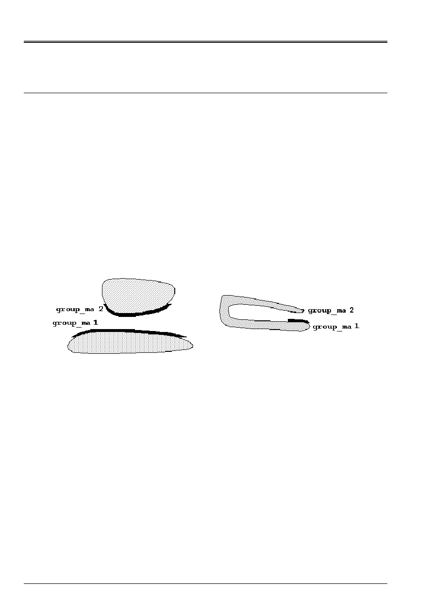
The contact will be done between

GROUP_MA_1

(or

MAILLE_1

) and it

GROUP_MA_2

(or

MAILLE_2

the statement of these two elements is essential.

Appear 3.1-a: Statement of surfaces of contact

Only the couples of surfaces declared here will be taken into account. If ever the contact were to be done
elsewhere, Code_Aster will not hold account of it.

All the loads of contact must be declared in the same one

AFFE_CHAR_MECA

, and

in the same key word contact. One will add as many occurrences of this key word there is
areas to be declared.

Example:

CHA = AFFE_CHAR_MECA (MODELE=MO,
DDL_IMPO=_F (GROUP_MA=' SOCLE',
DX=0.0,

DY=0.0,),

CONTACT= (_F (GROUP_MA_1 = “COTE_AB”,

GROUP_MA_2

“COTE_EF”,

METHOD

“LAGRANGIAN”,

PAIRING

“MAIT_ESCL”,),

_F (

GROUP_MA_1

“COTE_MP”,

GROUP_MA_2

“COTE_RS”,

METHOD

“LAGRANGIAN”,

PAIRING

“MAIT_ESCL”,

FRICTION

“COULOMB”,

COULOMB

2.0,),),);

Code_Aster

Version

6.4

Titrate:

Modeling of the contact

Date

04/11/03

Author (S):

S. LAMARCHE

Key

U2.04.04-A

Page

11/28

Instruction manual

U2.04 booklet: Nonlinear mechanics

HT-66/03/002/A

3.2

STAT_NON_LINE

and

DYNA_NON_LINE

[U4.51.03] and [U4.53.01]

STAT_NON_LINE

and

DYNA_NON_LINE

, key word

EXCIT

The statement of the load is very simple, since it is enough to give the name of the load built by

AFFE_CHAR_MECA

It is necessary of course, to regulate the parameters of specific pitches of time… to any mechanical study, without
to forget that the problem of contact is nonlinear.

Important remark:

One cannot use piloting in a problem of contact, nor linear search.

Example:

RESU = STAT_NON_LINE (MODELE=MO,
CHAM_MATER=CHMAT,
EXCIT=

(_F (CHARGE=CHA1,

FONC_MULT=F,),

_F (CHARGE=CONTACT,),),

COMP_INCR=_F (RELATION=' ELAS',

TOUT=' OUI',),

INCREMENT=_F (

LIST_INST=L_INST,

INST_FIN=1.5,
SUBD_PAS=2,
SUBD_PAS_MINI=1.E-3,),
NEWTON=_F (MATRICE=' TANGENTE',
REAC_ITER=1,),
CONVERGENCE=_F (RESI_GLOB_MAXI=1.E-8,
ITER_GLOB_MAXI=20,
ARRET=' OUI',),
ARCHIVAGE=_F (LIST_INST=L_INST,),);

Code_Aster

Version

6.4

Titrate:

Modeling of the contact

Date

04/11/03

Author (S):

S. LAMARCHE

Key

U2.04.04-A

Page

12/28

Instruction manual

U2.04 booklet: Nonlinear mechanics

HT-66/03/002/A

4 Modeling

The taking into account of the contact intervenes as of the creation of the mesh.
One will tackle in this part the questions useful to arise at the time of the stages of modeling.
This reflection relates to the mesh, but also the boundary conditions, the definition of surfaces of
contact and the taking into account of friction.

4.1

Mesh

4.1.1 Smoothness of the mesh

In the majority of the cases, it is preferable to refine the mesh in the areas of contact.
In particular in the curves, a fine mesh allows a better definition of the normal.
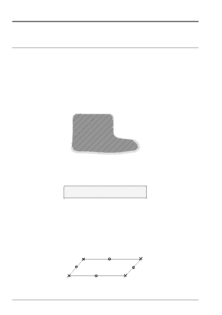
If the structure presents angles, a refined mesh will make it possible to round them slightly.

Appear 4.1.1-a: Mesh of an angular structure

On the other hand, on rigid levels, the processing of the contact is satisfied with a coarse mesh.

Appear 4.1.1-b: Mesh of a rigid plan

4.1.2 Choice of the finite elements

All the finite elements are compatible with calculations of contact.
The meshs of surfaces of contact are surface in dimension 3, linear in dimension 2. They
must be defined in the mesh, they are not automatically extracted from the meshs
voluminal by Code_Aster.
Case of the quadratic meshs

HEXA20

in 3D, and

QUAD9

in hulls:

Appear 4.1.2-a: Nets quadratic with its nodes node (X) and its nodes medium (O)

Code_Aster

Version

6.4

Titrate:

Modeling of the contact

Date

04/11/03

Author (S):

S. LAMARCHE

Key

U2.04.04-A

Page

13/28

Instruction manual

U2.04 booklet: Nonlinear mechanics

HT-66/03/002/A

In the case of the quadratic elements, Code_Aster imposes relations kinematics between
nodes mediums and the nodes nodes. Multipliers of Lagrange are applied to the nodes
mediums.
The first consequence is that the structure is more rigid.
Moreover, if boundary conditions (or of symmetry) are imposed on these elements, one needs them
to impose on the nodes nodes, but not on the nodes mediums not to create redundancies (two
multipliers of Lagrange on the same node).
In addition, the multiplier of Lagrange imply the use of larger matrices, and can
thus to harm the performances, and to pose problems of memory in the case of very large models.

4.1.3 Case of the beams

There is a problem specific to the beam, it does not have a single normal vector. The user must
to fix the direction of the normal with the key word

VECT_Y

The conditions of contact will be correctly taken into account only if the contact is done according to this
normal.
If these restrictions are incompatible with the restrictions of the problem, one can always net
beam in 3D.

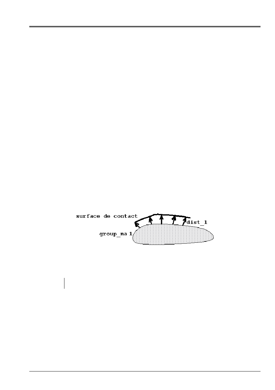
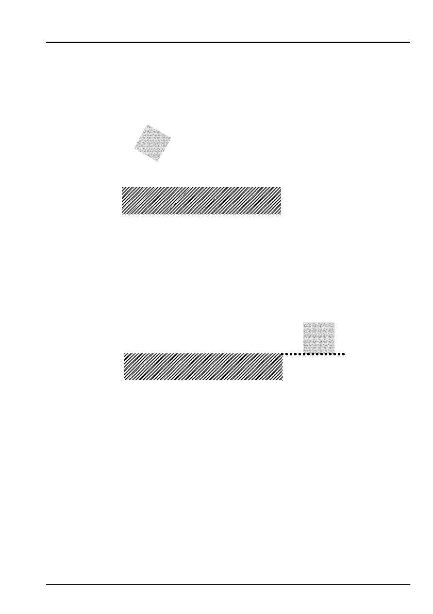
4.1.4 Thickness

material

Key words

DIST_1

and

DIST_2

allow to simulate defects of surface which are not

represented in the mesh. One adds on

GROUP_MA_1

(or

MAILLE_1

) for

DIST_1

and on

GROUP_MA_2

(or

MAILLE_2

) for

DIST_2

a thickness in the direction of the normal.

Thus,

DIST_1

> 0 correspond to a larger thickness,

DIST_1

< 0 with a smaller thickness.

Appear 4.1.4-a: Use of dist_1

Note:

This option replaces the mesh of defects of surface, but does not simulate the addition of
matter (inertia, arm of lever…).

Code_Aster

Version

6.4

Titrate:

Modeling of the contact

Date

04/11/03

Author (S):

S. LAMARCHE

Key

U2.04.04-A

Page

14/28

Instruction manual

U2.04 booklet: Nonlinear mechanics

HT-66/03/002/A

One can make use of it for the contact between hulls whose only average surface was with a grid. One can
also to make use of it to represent a broken surface.
During visualization, one does not see

DIST_1

and

DIST_2

. One can then see interpenetration then

that there is not (

DIST_1

DIST_2

<0) or not to see a contact whereas there is (

DIST_1

DIST_2

> 0).

dist_1

surfaces
of contact

dist_2

interpenetration

Appear 4.1.4-b: Visualization of an interpenetration

4.1.5

VECT_Y

VECT_Y

, key word of

AFFE_CHAR_MECA/CONTACT

allows to define a local reference mark on a surface

of contact. In this case, the local reference mark is built in the following way: the first V1 vector is
obtained by orthogonal projection of

VECT_Y

on the surface of the element considered, second V2 is

obtained by vector product of V1 with the normal vector NR.

Is also used it to give a normal to the beams.
In this case,

VECT_Y

is the vector, which, by vector product with the tangent vector with the beam,

give the normal to be used.

VECT_Y

Appear 4.1.5-a: Use of

VECT_Y

to define the normal in a beam

For other uses of

VECT_Y

, one can refer to U4 documentation of

AFFE_CHAR_MECA

Code_Aster

Version

6.4

Titrate:

Modeling of the contact

Date

04/11/03

Author (S):

S. LAMARCHE

Key

U2.04.04-A

Page

15/28

Instruction manual

U2.04 booklet: Nonlinear mechanics

HT-66/03/002/A

4.2

normals

It is imperative that the meshs of contact are defined so that the normals are
outgoing.
To have outgoing normals, the operator is used

MODI_MAILLAGE

, with the mots_clef

ORIE_PEAU_2D

ORIE_PEAU_3D

ORIE_NORM_COQUE

, according to modeling [U4.23.04].

Appear 4.2-a: the normal must be outgoing

Example:

MA = MODI_MAILLAGE (reuse=MA,
MAILLAGE=MA,
ORIE_PEAU_3D= (_F (GROUP_MA=' SURF_1',),

_F (GROUP_MA=' SURF_2',),),

MODELE=MO,);

4.3 Pairing

Two methods of pairing are available:

“NODAL”

“MASTER-SLAVE”

4.3.1 Method

“nodal”

Pairing is done between a node of surface slave and a main node of surface.

With each node slave, one pairs the main node nearest.
The relation of noninterpenetration uses by defect the normal with the mesh slave. Direction
of approach is either the normal with the mesh Master, or an arbitrary direction fixes (

VECT_NORM_2

Slave

Master

Vect_norm_2

Normal
Master

Appear 4.3.1-a: Example of use of

VECT_NORM_2

Code_Aster

Version

6.4

Titrate:

Modeling of the contact

Date

04/11/03

Author (S):

S. LAMARCHE

Key

U2.04.04-A

Page

16/28

Instruction manual

U2.04 booklet: Nonlinear mechanics

HT-66/03/002/A

Surface Master is that which comprises the most nodes (or if equality

MAILLE_2

GROUP_MA_2

Indeed, it is preferable that each main node is paired only with one node slave.
The Councils of use:
It is advised to have the compatible mesh and which remains compatible during calculation.
Method

“NODAL”

does not allow to correctly take into account great displacements.

One advises to use the method

“MASTER-SLAVE”

4.3.2 Method

“master-slave”

It is the advised method of pairing.
It is a pairing node-breakage. It is done between a node slave and a breakage Master.
The condition of contact is that the nodes slaves should not enter the meshs Masters.
It is noticed that the reverse is possible.
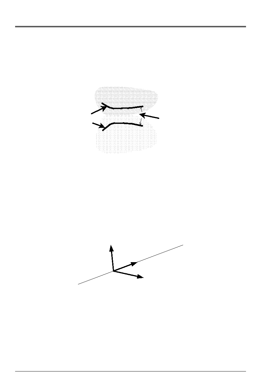
The relation of noninterpenetration uses by defect the normal with the mesh Master. One can also use
the average enters the normal to the mesh Master and the normal to the mesh slave.

Slave

Master

Average of
two directions

Normal
Master

Normal
slave

Appear 4.3.2-a: Example of use of the average between the direction

normal Master and that of the normal slave

Surface Master is that defined by

GROUP_MA_1

(or

MAILLE_1

), the mesh slave is that definite

GROUP_MA_2

(or

MAILLE_2

This method of pairing can be used in great displacements.

Main choice of surfaces and slaves:

If a surface is with a grid much more finely than the other, it is better that it is the slave for
to limit the interpenetration.
If one of surfaces is rigid, it is better that it is surface Master.
A surface Master can be paired on several surfaces slaves but a surface slave cannot
to correspond that to only one surface Master.

4.3.3

difficulties

For the methods

STRESS

and

LAGRANGE

, the conditions of contact are imposed by means of

multipliers of Lagrange on the nodes slaves (for the methods

STRESS

and

LAGRANGE

However one can put only one multiplier of Lagrange by node and direction.
The immediate consequences of this remark are:

a point should not belong to several surfaces slaves,

the points of surfaces slaves should not carry conditions of Dirichlet (

DDL_IMPO

FACE_IMPO

LIAISON_

…).

Code_Aster

Version

6.4

Titrate:

Modeling of the contact

Date

04/11/03

Author (S):

S. LAMARCHE

Key

U2.04.04-A

Page

17/28

Instruction manual

U2.04 booklet: Nonlinear mechanics

HT-66/03/002/A

4.3.4 Possible solutions

One can gather various surfaces of contact in only one. Surfaces of contact can be
angular. They can also be made up of disjoined surfaces of mesh.

surface slave

surface main

Appear 4.3.4-a: Example of angular surfaces of contact

One can exclude certain points from surfaces slaves. One uses for that the key words

SANS_NO

and

SANS_GROUP_NO

. This method is used for example to exclude from a surface slave them

nodes of an edge on which one imposed a boundary condition.

4.3.5 A particular case

It is possible that surface slave comes into contact with a main prolongation of surface.

surface slave

surface main

Appear 4.3.5-a: Example of contact with the main prolongation of surface

There are two solutions with this problem.
The first consists in choosing for the widest surface Master.
The second consists to widen surface Master and to take into account the other sides. (see
[Figure 4.3.4-a]).
This behavior can also disturb problems of more intricate geometry.

4.4

Boundary conditions

It is reminded the meeting that a node slave should not carry boundary condition (see paragraph
precedent).

Calculation must be able to be done even when the contact is removed. In dynamics, that does not impose
of particular stress. In statics, it is necessary that the structure does not hold only by the contact. One will make
thus attention to lock all the modes of rigid bodies.
To lock a rigid mode of body, it is enough to apply to the structure a displacement imposed (no one or
not) in the direction to be locked. Another method is to lock the mode of rigid body with one
comes out from low stiffness which too much will not disturb the result of calculation. This solution is not
alleviating and it is advised to check the results of calculation by making a parametric study on
stiffness of the spring.

Code_Aster

Version

6.4

Titrate:

Modeling of the contact

Date

04/11/03

Author (S):

S. LAMARCHE

Key

U2.04.04-A

Page

18/28

Instruction manual

U2.04 booklet: Nonlinear mechanics

HT-66/03/002/A

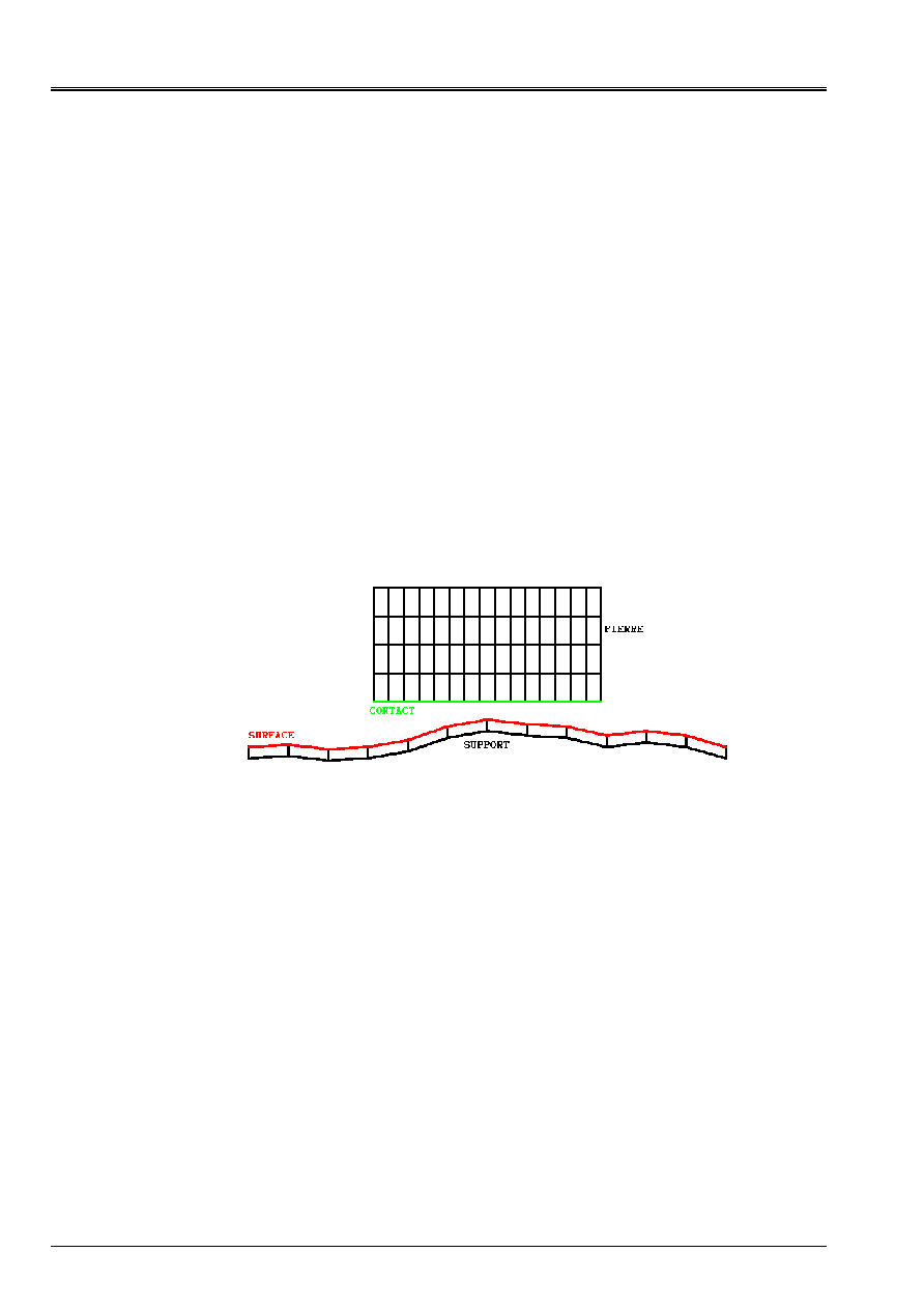
4.5 Surfaces

rigid

It may be that one of surfaces of the model is infinitely rigid.
One will even advise, in a preoccupation with a simplification of the problem, to regard as infinitely
rigid any surface much more rigid than the others.

The modeling of a rigid surface is done by locking its degrees of freedom with conditions
kinematics.
One can also increase his Young modulus to place it at at least an order of magnitude at
above Young moduli of other surfaces. But this last method is largely
disadvised because it can introduce numerical difficulties.

In the case of a problem of contact, rigid surface will be preferably surface Master.
The plane parts of rigid surface can be modelized very coarsely. On the other hand, for
a better definition of the normals, it is advised to net the curved areas finely.

If rigid surface is surface slave, one will not be able to deal with the problem while posing
conditions kinematics….

4.5.1 Extracts of a command file comprising a rigid surface

…
MODE=AFFE_MODELE (MAILLAGE=MA,

VERIF=' MAILLE',
AFFE= (_F (TOUT=' OUI',

PHENOMENON = “MECHANICAL”,
MODELING = “D_PLAN”),),);

MA=MODI_MAILLAGE (REUSE=MA,

MAILLAGE=MA,
MODELE=MODE,
ORIE_PEAU_2D=_F (GROUP_MA= (“CONTACT”, “SURFACE”)),
INFO=2);

…
CH=AFFE_CHAR_MECA (MODELE=MODE,

DDL_IMPO= (_F (GROUP_MA = “SURFACE”, DX = 0., DY = 0. ),),
CONTACT=_F (REAC_GEOM=' CONTRÔLE',

NB_REAC_GEOM=2,
GROUP_MA_1=

“SURFACE”,

GROUP_MA_2=

“CONTACT”,

METHODE=' LAGRANGIEN',
FRICTION = “COULOMB”,

PESANTEUR= (9.8, 0., - 1., 0.),);

Code_Aster

Version

6.4

Titrate:

Modeling of the contact

Date

04/11/03

Author (S):

S. LAMARCHE

Key

U2.04.04-A

Page

19/28

Instruction manual

U2.04 booklet: Nonlinear mechanics

HT-66/03/002/A

RESU=DYNA_NON_LINE (

MODELE=MODE,

CHAM_MATER=CHMAT,
EXCIT=_F (CHARGE=CH,),
ETAT_INIT=_F (QUICKLY = VIT_0),
COMP_INCR=_F (RELATION=' ELAS',

DEFORMATION=' SIMO_MIEHE',
TOUT=' OUI',),

INCREMENT=_F (LIST_INST=L_INST,

SUBD_PAS=4,
SUBD_PAS_MINI=1.E-17,
COEF_SUBD_PAS_1=1.0,),

HHT=_F (ALPHA=-0.05),
NEWTON=_F (REAC_ITER=1,

MATRICE=' TANGENTE',),

CONVERGENCE=_F (RESI_GLOB_RELA=1.E-06,

ITER_GLOB_MAXI=25,
ARRET=' OUI',),

ARCHIVAGE=_F (ARCH_ETAT_INIT=' OUI',

PAS_ARCH=100,),);

4.6

friction

The modeling of friction in 3D is a rather delicate thing. Also, if in a study 3D it
coefficient of friction is very low, it is advised to neglect frictions.

For a study with friction, it is advised to initially treat it without friction so
to give an order of magnitude of the answer and with the aim of introduce the difficulties ones
after the others.

5 Calculations

It is strongly advised to read U4 documentations of

AFFE_CHAR_MECA

and of

STAT_NON_LINE

DYNA_NON_LINE

The contact is treated like a load in the equation of dynamics.
The difficulties encountered during calculation are not obligatorily due to the contact.
The processing of the contact is one of nonthe linearities of the problem. The problem can comprise others
not linearities.

5.1

Taking into account of the contact friction

In the operator

AFFE_CHAR_MECA

, one is brought to choose the method of calculation of the contact. Three

methods are possible:

“FORCED”

“LAGRANGE”

and

“PENALIZATION”

5.1.1

“FORCED”

It is based on the algorithm of the active stresses (see documentations R of reference for
more details).
It is an exact method. It uses the multipliers of lagrange. There is not interpenetration enters
structures.
One cannot use it with friction.

Code_Aster

Version

6.4

Titrate:

Modeling of the contact

Date

04/11/03

Author (S):

S. LAMARCHE

Key

U2.04.04-A

Page

20/28

Instruction manual

U2.04 booklet: Nonlinear mechanics

HT-66/03/002/A

5.1.2

“LAGRANGE”

It is an exact method.
It uses the multipliers of Lagrange and an algorithm equivalent to that of the method

STRESS

This method allows the use of friction.

5.1.3

“PENALIZATION”

This method treats penalized friction (coefficient AND), but the contact is is penalized
(coefficient IN) is treated by multiplier of lagrange. It is the user who decides (if it provides IN
contact is penalized, if it does not provide it the contact is treated by multiplier of Lagrange).

5.1.3.1 Choice of the coefficients of penalization

The choice of the coefficients of penalization is a delicate choice. More especially as the result obtained is
very dependant on this coefficient.

The higher the coefficient of penalization will be, the more the result will be close to the exact result. But one
too high coefficient of penalization (compared to the other stiffnesses of the problem) can induce
numerical problems.

In practice, one can start with a coefficient of the same smallest order of magnitude as
Young modulus of the problem. Then, one gradually increases it (of a factor 10 for example) until
the stabilization of the results.

Note:

For the coefficient IN, one can validate the result of calculation by checking that the interpenetration is not
not too large. One can sometimes increase it up to 10

to 10

time the smallest Young modulus.

5.1.3.2 Advantages and disadvantages

The penalization does not induce discontinuity of the fields speed. What can be an advantage in
a calculation in dynamics.
However it is not exact because it authorizes the interpenetration, and the results are very
dependant on the coefficients of penalization.

5.1.4 Remarks

Here a list of remarks to contribute to the choice of the method.
For an elastic design, method

“LAGRANGE”

(or of the active stresses if there is not

friction) is faster.
The penalization gives results very dependant on the coefficients of penalization.
In the case of a calculation with penalized friction, one can check his results while testing with one
another method.
In the case of a penalized normal contact, a checking can be the depth of interpenetration.
It should not be too large.
It is reminded the meeting that one can use only one method for the conditions of contact of same
calculation.
In 2D, one will use rather

“LAGRANGE”

“FORCED”

5.2 Friction

When friction is activated, it is necessary to provide a coefficient of Coulomb friction in all the cases. In
3D in surface contact (meshs 2D), it is also necessary to fix it

COEFFICIENT_MATR_FROT

(see

U4 documentation). And in the case of a calculation with penalization, it is necessary to give AND (see § penalization).

Code_Aster

Version

6.4

Titrate:

Modeling of the contact

Date

04/11/03

Author (S):

S. LAMARCHE

Key

U2.04.04-A

Page

21/28

Instruction manual

U2.04 booklet: Nonlinear mechanics

HT-66/03/002/A

5.3 Interpenetration

At the end of calculation, one can observe an interpenetration of the structures. It can be due to several
reasons.

5.3.1 Calculation

penalized

In the case of a penalized calculation, there is always interpenetration at the time of the contact, since them
forces of contact become active when the play is negative.
This interpenetration is weaker if the normal coefficients of penalization (IN) are higher.

5.3.2 Dissymmetry Master/slave

One can have an interpenetration of the main nodes in surfaces slaves. For some
geometries, this phenomenon can become awkward (too major interpenetration, or penetration
supplements of a main relief of the mesh in a surface slave). It is enough to net them more finely
surfaces slaves in the areas concerned.

surface slave

surface
Master

Appear 5.3.2-a: Example of interpenetration due to dissymmetry Master/slave

5.3.3 Visualization

One will of course pay attention to the artefacts of visualization.
Like one saw in the § Epaisseur material, if the key words are used

DIST_1

and

DIST_2

, one can

then to see interpenetration whereas there is not (

DIST_1

DIST_2

<0) or not to see a contact

whereas there is (

DIST_1

DIST_2

> 0).

During a visualization, one is brought to choose a scale factor. This factor multiplies them
displacements and makes it possible the user to better observe them. In the case of a study with contact, it
is necessary to put this scale factor at 1.
If this factor is higher than 1, one can observe much interpenetration where there is not
all.

5.4

calculation

Calculation is done with

STAT_NON_LINE

DYNA_NON_LINE

. It is advised to read documentations

U4 associated with its operators. One will be able to also refer to the documents of the Aster formation.
At the time to make the choices of the various options, one will not forget that the problem of contact is
nonlinear.
One will put the question to know if one works into small or in great displacements.
It is reminded the meeting that the options of linear search and that of piloting are not possible with
contact.

Code_Aster

Version

6.4

Titrate:

Modeling of the contact

Date

04/11/03

Author (S):

S. LAMARCHE

Key

U2.04.04-A

Page

22/28

Instruction manual

U2.04 booklet: Nonlinear mechanics

HT-66/03/002/A

5.5 Large

displacements

One considers in this paragraph, the problems in great displacements.
The detection of the contact is done according to the geometry of the structure and the relations of not
interpenetration are based on the directions of the normals. In the event of great displacements, one thus has
need to work on a reactualized geometry.
One does not speak here about great deformations. The possibility or not of treating the great deformations
does not depend on the contact.
In addition, one will choose parameters of calculation in the operator

STAT_NON_LINE

DYNA_NON_LINE

compatible with a calculation in great displacements.

5.5.1 Seek

The search of pairing is done either in the direct vicinity of the node of preceding contact, or
on all the structure. In the event of great displacements, one uses search on all the structure.

5.5.2 Reactualization

geometry

According to if one works into large or small displacements, one will choose a reactualization of
different geometry.

REAC_GEOM=' SANS'

In this case, one works on the initial geometry. One uses this choice only for

studies in small displacements.

For great displacements, one uses one of the two other choices.
The choice by defect is:

REAC_GEOM=' AUTO'

. The reactualization of the geometry is automatic. It is done until satisfying

a geometrical criterion of convergence.
One can also impose the iteration count with:

REAC_GEOM=' CONTRÔLE'

This number is specified

with

NB_REAC_GEOM=n

Value 1 indicates that with convergence, one reactualizes the geometry and one passes to the pitch of
charge according to.

Value 2 indicates that to convergence, one does not pass to the pitch of load according to.
One reactualizes the geometry and one reiterates until convergence.

The value n>2 indicates that one makes N cycles reactualization geometrical-iterations until
convergence.

5.6

The dynamic case

The preceding remarks are valid in statics (

STAT_NON_LINE

) and in dynamics

(

DYNA_NON_LINE

One will draw the attention to some points particular to dynamic calculations.
In a problem dealt with with multipliers of Lagrange, at the time of the impact speed is
discontinuous. Acceleration is thus not defined in this moment.
This remark can be in the beginning strong oscillations of the answer, or a strong sensitivity to
diagram of calculation used and with the pitch of time. One strongly advises to start with the pitch of
time which observes the condition of current (time put by the wave to cross an element) then
to test several pitches of smaller or larger times.

One can attenuate the oscillations by using a diagram which generates numerical damping.
In the case of a penalized calculation, it is not there a jump speed. This method east can be more
correct on a mathematical level, but it generates it also oscillations of the answer to
moment of the contact.

Code_Aster

Version

6.4

Titrate:

Modeling of the contact

Date

04/11/03

Author (S):

S. LAMARCHE

Key

U2.04.04-A

Page

23/28

Instruction manual

U2.04 booklet: Nonlinear mechanics

HT-66/03/002/A

6 Others

methods

In this part, one presents two other methods available in Code_Aster to treat it
contact. Their applicability is more restricted (penalized calculation and specific contact) but they
have some characteristics which can be useful and which are exposed Ci below.

6.1

DYNA_TRAN_MODAL

For the use of this operator, one advises the reading of U4 documentation.
For postprocessing, one will read in particular U4 documentation of

POST_DYNA_MODA_T

6.1.1 Presentation

DYNA_TRAN_MODAL

calculate a transitory dynamic response on truncated modal basis. It allows

taking into account of contact-friction.
The use of this operator supposes that modal calculation is already made.

DYNA_TRAN_MODAL

propose several methods of calculation. The explicit methods will be used

(

“EULER”

“DEVOGE”

“ADAPT”

) to treat the contact.

One enters the data relating to contact-friction under the key word

“SHOCK”

6.1.2 Processing of the contact

It is about a specific contact, penalized, in small displacements.
One can take into account the damping of shock. (It is reminded the meeting that the effect of this damping
depends on the pitch of time.).
The user potentially provides the couples of nodes in contact, as well as the coefficients of
penalization (IN and AND) and of damping.

6.1.3 Modeling

6.1.3.1 Thickness

material

It corresponds to the thickness material of the loads of contact.
It is noticed that a negative initial play is equivalent to a prestressing.

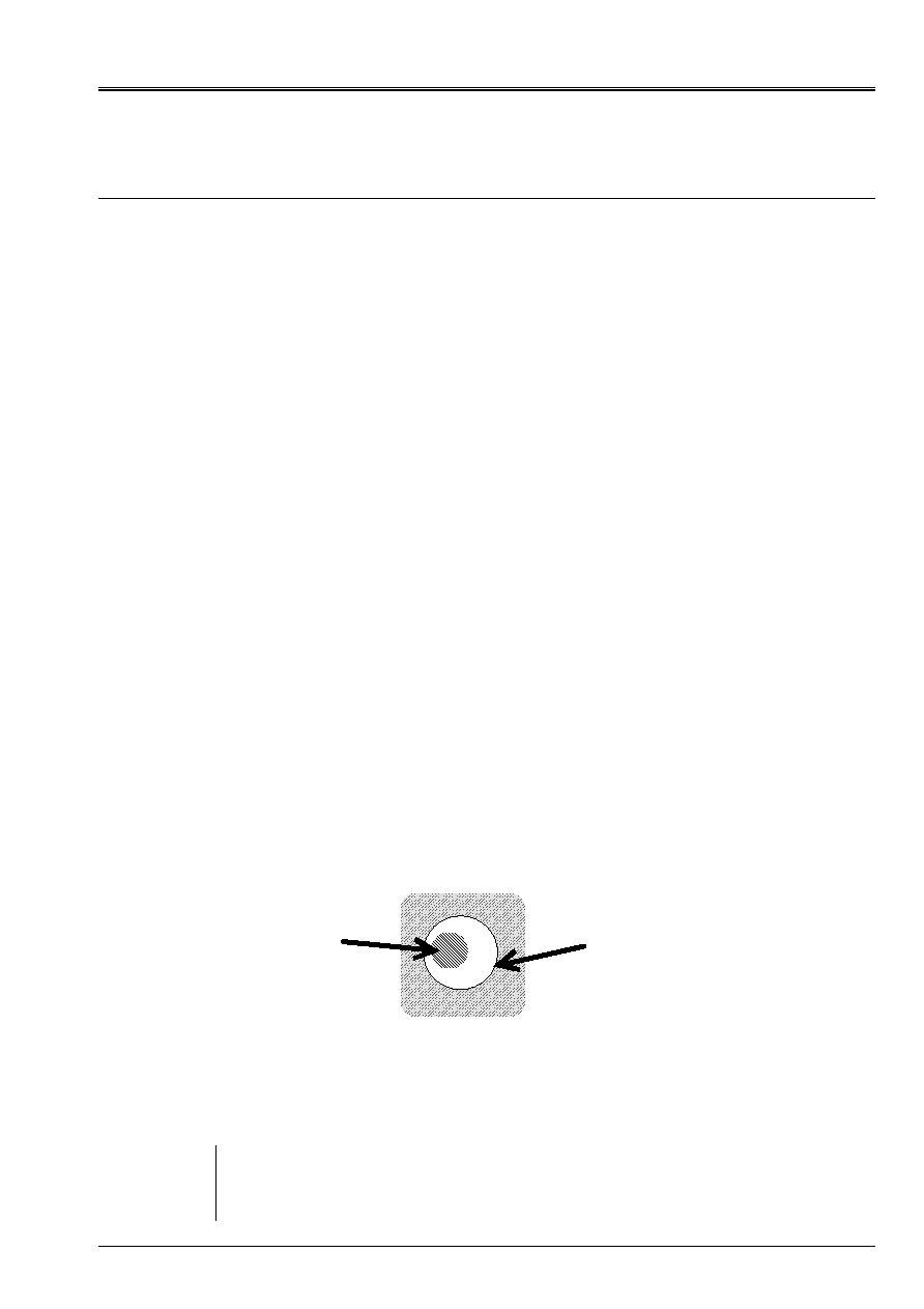
6.1.3.2 Obstacles nonwith a grid

It is possible to take account of not modelized rigid surfaces. They are defined by

DEFI_OBSTACLE

. They lock the displacement of a point inside a defined pre curve, or

between two plans.

Structure
studied

obstacle
defined by
DEFI_OBSTACLE

Appear 6.1.3.2-a: Example of use of

DEFI_OBSTACLE

These surfaces are infinitely rigid, but one can affect a flexibility to them by the means of
coefficients of penalization.

Note:

One can make evolve/move these obstacles during calculation according to profiles' determined with
operators

POST_USURE

and

MODI_OBSTACLE

. On this point, it is advised to consult them

U4 documentations of

POST_USURE

and of

MODI_OBSTACLE

, to see on which types

of study these calculations are applicable.

Code_Aster

Version

6.4

Titrate:

Modeling of the contact

Date

04/11/03

Author (S):

S. LAMARCHE

Key

U2.04.04-A

Page

24/28

Instruction manual

U2.04 booklet: Nonlinear mechanics

HT-66/03/002/A

6.1.4 The Councils

of use

The choice of the coefficients of penalizations is in the same way made that for the penalized method of
loads of contact.
The modal base is worked out and one keeps it in an Aster base. Much time then is gained
on transitory calculations.
If the problem includes/understands rigid surfaces, or surfaces of contact which do not move, one
can modelize them with

DEFI_OBSTACLE

6.1.5 Postprocessing

The components of the results are directly accessible by

RECU_FONCTION

DYNA_TRAN_MODAL

have postprocessing specific. They make it possible to make studies

of impact or studies of wear. They are accessible from

POST_DYNA_MODA_T

and its options

“IMPACT”

“WEAR”

. One will refer to U4 documentation of

POST_DYNA_MODA_T

for the list

postprocessing included/understood in these two options.

6.1.6 Assessment

This method of the processing of the contact is limited to the specific studies of contact, penalized, into small
displacements.
Put aside nonlocal linearities envisaged by the operator (like the specific shocks), the problem
must be linear, since calculation is made starting from the modal base.

In its field of application, it has the advantage of taking into account damping and of laying out
of a rich postprocessing.
The truncation of the modal base makes it possible to make fast transitory calculations. One will make however
attention to choose the size of the base used well. In the case of a study with shock, one can be
brought to go up rather high in frequency.
The creation of obstacles except mesh can represent an important gain of size for the model.

6.1.7 One

example

TRANGENE = DYNA_TRAN_MODAL (

METHOD = “euler”,

MASS_GENE

MASSEGEN,

RIGI_GENE

RIGIGEN,

EXCIT

(_F (VECT_GENE

FORC1,

FONC_MULT

FONC1,),

_F (VECT_GENE = FORC2,
FONC_MULT

FONC2,),),

INCREMENT

_F (INST_INIT

=0.,

INST_FIN

2.5,

NOT

4.E-5,),

SHOCK

(_F (

GROUP_NO_1

“A”,

GROUP_NO_2

“AA”,

OBSTACLE

OBST1,

NORM_OBST

(0., 1., 0.,),

PLAY = 0.1,

RIGI_NOR

1.E11,

RIGI_TAN

1.5E8,

COULOMB

0.6,),

_F (

GROUP_NO_1

“B”,

OBSTACLE

OBST2,

NORM_OBST

(0., 1., 0.,),

PLAY

0.05,

RIGI_NOR

2.E9,

RIGI_TAN

2.E7,

COULOMB

0.5,),),);

Code_Aster

Version

6.4

Titrate:

Modeling of the contact

Date

04/11/03

Author (S):

S. LAMARCHE

Key

U2.04.04-A

Page

25/28

Instruction manual

U2.04 booklet: Nonlinear mechanics

HT-66/03/002/A

6.2

DIS_CONTACT

Elements

DIS_CONTACT

allow to modelize a specific contact, penalized, into small

displacements. They are discrete elements.
Contrary to the preceding chapter, calculation is then direct (operators

STAT_NON_LINE

DYNA_NON_LINE

Elements

DIS_CONTACT

are generally elements with two nodes, present in

mesh. They connect the two points which will be potentially in contact during calculation. There is too
elements with a node, for which it is necessary to affect a play in the normal direction of shock (confused
with the local axis X).

These elements have many characteristics which one declares in

DEFI_MATERIAU

One advises the reading of Doc. U4 of

DEFI_MATERIAU

to obtain the exhaustive list of these

parameters and their definition.
The interest of these elements is their great richness of behavior. One can give them laws of
behavior particular (elastoplastic, dependant on time…).
Of course, for multiplying the use of these parameters, it will be necessary to raise the question of
to know which have a relevant direction for the study.

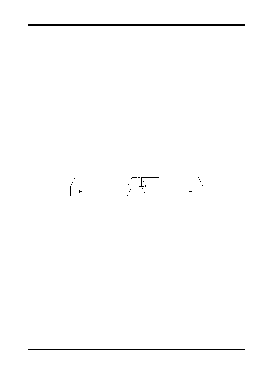
In the command file according to, one uses them to calculate the contact between two beams
modelized in 3D.

6.2.1 Example of command file

Elements of contact

ACHOC 1 to 4

POU1

POU2

Appear 6.2.1-a: Mesh of the study

# Construction of the mesh

MAIL=LIRE_MAILLAGE ();
MAIL=DEFI_GROUP (reuse =MAIL,
MAILLAGE=MAIL,
CREA_GROUP_MA=_F (NOM=' ACHOC',
UNION= (“ACHOC1”, “ACHOC2”, “ACHOC3”, “ACHOC4”,),),
CREA_GROUP_NO=_F (TOUT_GROUP_MA=' OUI',),);

Beams POU1 and POU2 are in 3D, whereas the elements of shock are the discrete ones. One them

allot characteristics thanks to the operator

DEFI_MATERIAU

In this study, one chose

to take account of a damping (which acts that there is contact or not). One indicates also the coefficient of
penalization of the shock.
(It is reminded the meeting that the effect of damping depends on the pitch on time.)

Code_Aster

Version

6.4

Titrate:

Modeling of the contact

Date

04/11/03

Author (S):

S. LAMARCHE

Key

U2.04.04-A

Page

26/28

Instruction manual

U2.04 booklet: Nonlinear mechanics

HT-66/03/002/A

MODELE=AFFE_MODELE (MAILLAGE=MAIL,
AFFE= (_F (GROUP_MA= (“POU1”, “POU2”,),
PHENOMENE=' MECANIQUE',
MODELISATION=' 3d',),
_F (GROUP_MA= (“ACHOC1”, “ACHOC2”, “ACHOC3”, “ACHOC4”,),
PHENOMENE=' MECANIQUE',
MODELISATION=' DIS_T',),),);

ACIER=DEFI_MATERIAU (ELAS=_F (E=200000000000.0,
NU=0.3,
RHO=7800.0,),);
AMOR=DEFI_MATERIAU (DIS_CONTACT=_F (RIGI_NOR=1000000000.0,
AMOR_NOR=5.0,),);

CHMAT=AFFE_MATERIAU (MAILLAGE=MAIL,
AFFE= (_F (GROUP_MA=' POU1',
MATER=ACIER,),
_F (GROUP_MA=' POU2',
MATER=ACIER,),
_F (GROUP_MA= (“ACHOC1”, “ACHOC2”, “ACHOC3”, “ACHOC4”,),
MATER=AMOR,),),);

# For the correct operation of the operator

DYNA_NON_LINE

, one must indicate a matrix of stiffness

for the discrete elements. One chooses null coefficients not to disturb the continuation of calculation.

CARELEM=AFFE_CARA_ELEM (MODELE=MODELE,
DISCRET=_F (GROUP_MA= (“ACHOC1”, “ACHOC2”, “ACHOC3”, “ACHOC4”,),
CARA=' K_T_D_L',
VALE= (0.0, 0.0, 0.0,),),);

….

# The elements dis_contact have a relation of behavior

“DIS_CHOC”

that one informs in

COMP_INCR

. Whereas the beams have an elastic behavior.

U0=DYNA_NON_LINE (MODELE=MODELE,
CHAM_MATER=CHMAT,
CARA_ELEM=CARELEM,
EXCIT= (_F (CHARGE=CONDLIM,),),
COMP_INCR= (_F (RELATION=' ELAS',
DEFORMATION=' PETIT',
GROUP_MA= (“POU1”, “POU2”,),),
_F (RELATION=' DIS_CHOC',
GROUP_MA= (“ACHOC1”, “ACHOC2”, “ACHOC3”, “ACHOC4”,),),),
ETAT_INIT=_F (VITE=VITINI,),
INCREMENT=_F (LIST_INST=L_INST,
SUBD_PAS=3,
SUBD_PAS_MINI=1e-08,),
NEWMARK=_F (ALPHA=0.25,
DELTA=0.5,),
NEWTON=_F (MATRICE=' TANGENTE',
REAC_ITER=1,),
SOLVEUR=_F (METHODE=' MULT_FRONT',),
CONVERGENCE=_F (RESI_GLOB_RELA=1e-05,
ITER_GLOB_MAXI=60,
ARRET=' OUI',),
ARCHIVAGE=_F (LIST_INST=L_ARCH,),);

Code_Aster

Version

6.4

Titrate:

Modeling of the contact

Date

04/11/03

Author (S):

S. LAMARCHE

Key

U2.04.04-A

Page

27/28

Instruction manual

U2.04 booklet: Nonlinear mechanics

HT-66/03/002/A

7 Bibliography

[1]

NR. TARDIEU: Code_Aster, documentation Reference, [R5.03.50], 2001

[2]

P. MASSIN: Code_Aster, documentation Reference, [R5.03.51], 2001

[3]

X. DESROCHES: Code_Aster, documentation Use, [U4.44.01], 2003

[4]

E. BOYERE: Code_Aster, documentation Use, [U4.53.21], 2003

[5]

V. CANO: Code_Aster, documentation Use, [U4.51.03], 2003

[6]

G. DEVESA: Code_Aster, documentation Use, [U4.51.01], 2003

[7]

E. BOYERE: Code_Aster, documentation Use, [U4.84.02], 2003

[8]

J.P. LEFEBVRE: Code_Aster, documentation Use, [U4.43.01], 2003