Conservation of Mass

Figure 4.1: Differential Control Volume

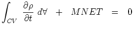
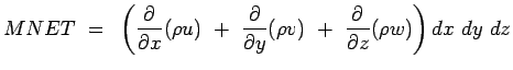
We derive the equation for mass conservation by considering a differential control volume at P(x,y,z)as shown in Fig.4.1. Let the dimensions of the volume be dx, dyand dz and velocity components at P be u,v and w. Assuming that the mass flow rate is continuous across the volume we can calculate the mass flow rates at the various faces of the cell by a Taylor Series expansion as we had done previously (Eqn. 2.5). Accordingly we have,

$$ML =\left[ \rho u - {\partial \over {\partial x}}(\rho u)  dx\ri... ...z; MR =\left[ \rho u + {\partial \over {\partial x}}(\rho u)  dx \right] dy dz$$

$$MB =\left[ \rho v - {\partial \over {\partial y}}(\rho v)  dy\ri... ...z; MT =\left[ \rho v + {\partial \over {\partial y}}(\rho v)  dy \right] dx dz$$

$$MA =\left[ \rho w - {\partial \over {\partial z}}(\rho w)  dz\ri... ...y; MF =\left[ \rho w + {\partial \over {\partial z}}(\rho w)  dz \right] dx dy$$ (4.1)

The net mass flow rate into the control volume as a consequence is given by,

$$MNET =  MR - ML + MT - MB + MA - MF$$ (4.2)

Applying the Reynolds transport theorem for mass (Eqn. 3.30) will give,

$${\int_{CV} {{\partial \rho} \over {\partial t}} d \forall}  +  MNET  =  0$$ (4.3)

From Eqn.4.1 and 4.2 we have,

$$MNET = \left( {\partial \over {\partial x}}(\rho u) + {\partial ... ...\partial y}}(\rho v)  + {\partial \over {\partial z}}(\rho w) \right) dx dy dz$$ (4.4)

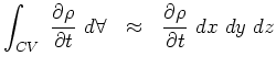
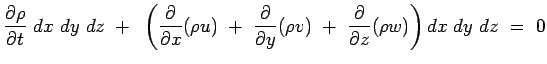
Further in Eqn.4.3 noting that the control volume is tiny, the integral can be approximated as

$${\int_{CV} {{\partial \rho} \over {\partial t}} d \forall}  \approx  {{\partial \rho} \over {\partial t}} dx dy dz$$ (4.5)

The Reynolds Transport Theorem thus gives,

$${{\partial \rho} \over {\partial t}} dx dy dz + \left( {\partial ... ...tial y}}(\rho v)  + {\partial \over {\partial z}}(\rho w) \right) dx dy dz = 0$$ (4.6)

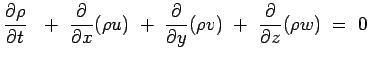
Cancelling out dx dy dz, we have,

$${{\partial \rho} \over {\partial t}}  + {\partial \over {\partial... ...rtial \over {\partial y}}(\rho v)  + {\partial \over {\partial z}}(\rho w) = 0$$ (4.7)

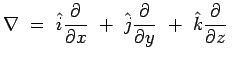
Eqn. 4.7 is known as the Continuity Equation. Note that it is a very general equation with hardly any assumption except that density and velocities vary continually across the element we have considered.

If we now bring in the gradient operator, namely,

$$\nabla = \hat{i}{\partial \over {\partial x}} + \hat{j}{\partial \over {\partial y}}  + \hat{k}{\partial \over {\partial z}}$$ (4.8)

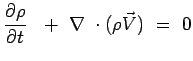
and represent velocity as a vector,

$$\vec{V} = \hat{i}u + \hat{j}v + \hat{k}w$$ (4.9)

Then the Continuity Equation can be written in a compact manner as

$${{\partial \rho} \over {\partial t}}  + \nabla \cdot (\rho \vec{V}) = 0$$ (4.10)

Written in this form it enables one to consider any other system of coordinates with ease.

(c) Aerospace, Mechanical & Mechatronic Engg. 2005
University of Sydney