Continuity Equation in Cylindrical Polar Coordinates

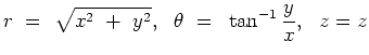
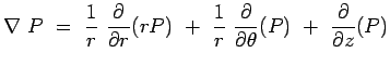
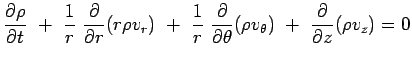
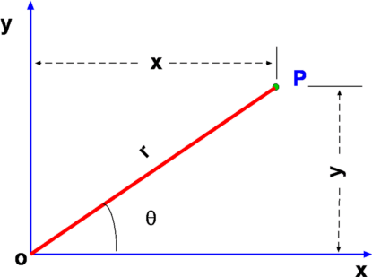
We have derived the Continuity Equation, 4.10 using Cartesian Coordinates. It is possible to use the same system for all flows. But sometimes the equations may become cumbersome. So depending upon the flow geometry it is better to choose an appropriate system. Many flows which involve rotation or radial motion are best described in Cylindrical Polar Coordinates. Let us now write equations for such a system. In this system coordinates for a point P are $r, \theta$ and

, which are indicated in Fig.4.2. The velocity components in these directions respectively are $v_r, v_\theta$ and

. Transformation between the Cartesian and the polar systems is provided by the relations,

$\displaystyle r = \sqrt{x^2 + y^2}, \theta = \tan^{-1}{y \over x}, z=z$

(4.11)

The gradient operator is given by,

$\displaystyle \nabla P = {1 \over r} {\partial \over \partial r} (rP) + {1 \over r} {\partial \over \partial \theta}(P) + {\partial \over \partial z}(P)$

(4.12)

As a consequence the continuity equation becomes,

$\displaystyle {{\partial \rho}\over {\partial t}} + {1 \over r} {\partial \over... ...over \partial \theta}(\rho v_\theta) + {\partial \over \partial z}(\rho v_z)=0$

(4.13)

Figure 4.2: Cylindrical Polar Coordinate System