Periodic loading

When the load torque is not constant, but varies cyclically in some manner with period   t_o as shown, it is usual to define an equivalent constant load torque,   T_e , which has the same life reduction effect on the motor as has the cycle; thus :-

( 3 )       T_e^m t_o   =   ∫₀^t_o T^m dt
                              where   m is a constant, noting that, as   m --> ∞ then   T_e --> T_max.
Since motor speed is essentially constant, power may be substituted for torque here.

The rationale behind ( 3) is the approximate relation :   life∗load^m ≈ constant, which many components and machines are found to follow. Thus   m ≈ 3 for rolling element bearings,   m ≈ 12 for V-belts, and so on. Electric motor life depends on a complex interaction of electrical and thermal phenomena, as has been seen, and there is thus no real justification for adopting the traditional RMS value of   m = 2 - though the concept of RMS current rather than load may be appropriate. Rather, manufacturer's data indirectly suggests a value of   m ≈ 5.

If the torque consists of a sinusoid, of amplitude   T_a   { nomenclature explanation} superimposed on a mean component   T_m as sketched, where   T_a ≤ T_m , then ( 3) gives the equivalent load   T_e as
            ( T_e )^m   =   ( ¹/_2π ) ∫₀^2π ( T )^m dθ   =   ( ¹/_2π ) ∫₀^2π( T_m + T_a sinθ )^m dθ     - or, normalising

( 3a)       ( T_e / T_m )^m   =   ( ¹/_2π ) ∫₀^2π ( 1 + λ.sinθ )^m dθ       where   λ = T_a / T_m
                                            =   Σ_q=0^{m div 2} [ m! ( ^λ/₂ )^2q ] / [ ( m -2q )! ( q! )² ]       for integer   m, and
                                            =   1 + 5 λ² + ¹⁵/₈ λ⁴       for   m = 5   for example.

The choice of a motor suitable to drive a cyclic load is based on the motor's full load torque equalling or exceeding the load's equivalent constant torque   T_e , whilst ensuring that the breakdown torque substantially exceeds the peak torque of the load cycle. The effect of system inertia in reducing speed fluctuations, and hence the torque variations experienced by the motor, is demonstrated in the Problems which follow.

AS 1359 classifies eight duty types, S1 through S8, three of which are illustrated.

S1 - continuous maximum duty

This has already been discussed.

S2 - short time duty

The motor is loaded by a uniform torque   T for a short period   t* = 10, 30, 60 minutes etc, and thereafter it is shut down until its temperature returns to ambient.
ABB recommends that :
      if   t* = 30 minutes, then   T_e = T/1.2
      if   t * = 60 minutes, then   T_e = T/1.1

S3 - intermittent periodic duty

The cyclic duration factor (cdf) is defined as   t*/ t_o in which the period   t_o is 10 minutes. Again the motor is de-energised when off-loaded.
ABB recommendations correspond to   m ≈ ¹⁶/₃ in ( 3) ie.   T_e /T = ( cdf )^1/m ; it is for this reason that m ≈ 5 is suggested above - at least for preliminary estimation purposes pending confirmation from the manufacturer - though S3 is not a cycle as conceived in ( 3) since the motor is shut down during part of the cycle and there is no fan cooling while shut down.

When a motor is started frequently, in a situation similar to S3 but with a period less than 10 minutes, the temperature build-up due to frequent acceleration may be significant even although the eventual load is negligible. ABB suggests that the load be increased by the factor :-

( 3b)       ( 1 - ( 1 + J_L / J_M ) ( x / x_max ) ) ^-1/2   ≥   1
                        where   x is the number of starts per hour,   x_max is the maximum allowable number of starts per hour and   J_M is the motor inertia (both of which are tabulated above), and J_L is the load inertia referred to the motor shaft (see below).

Acceleration

Squirrel cage motors suffer from drawing high starting current - typically some 6-8 times full load current - so I²R losses at starting are much greater than the full load losses which the cooling system can handle on a continuous basis. Lengthy starting periods thus cause early failure. Star -delta starting reduces initial current but is generally not recommended, for quadratic loads at least; direct on -line (DOL) starting is usually the more favoured. The starting period for a motor -driven load may be found from the equation of motion of the system referred to the motor shaft :-
            T_net   =   T_M - T_L   =   J dω/dt   ;       ω = 2πn
where J is the system inertia referred to the motor shaft ie.   J = J_motor + J_load /R² etc.
Integrating this yields the acceleration time, Δ_t , to reach running speed   n_r from rest :-

( 4 )       Δ_t   =   2π J ∫₀^n_r ( 1 / T_net ) dn

Although this period tends theoretically to infinity, a slight reduction of the upper limit enables realisitic integration to be carried out, possibly by the graphical techniques of the Appendix. The reduction is excusable in view of the full-load current being so much lower than starting, and the questionable applicability of the motor's steady state characteristic to a transient analysis.

The starting period so calculated must not exceed the maximum allowable starting time for a DOL-started motor laid down by the manufacturer - refer to the table above. Although star-delta starters allow about three times the starting period permitted with DOL, torques are reduced. If the starting time for an intended motor is excessive - that is the system inertia is relatively large - then consideration should be given to a clutch or hydraulic coupling, rather than opting for a larger motor. As will be seen, these devices isolate the motor from high inertia loads thus allowing the motor to accelerate quickly.

Hydraulic couplings

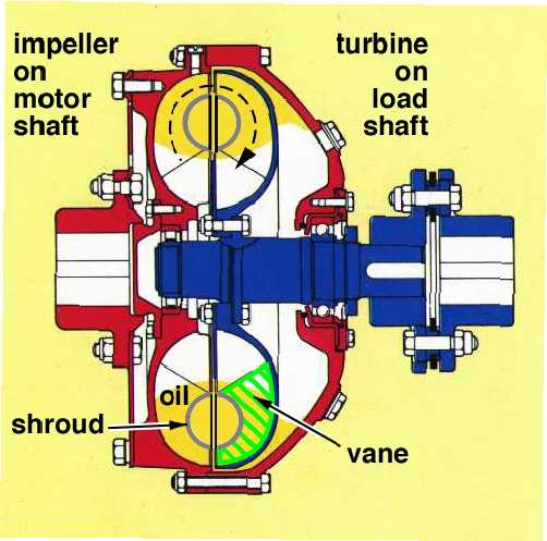
A hydraulic coupling consists of an impeller (pump) and a turbine, each equipped with multiple vanes and each mounted on a separate shaft in a casing which is partially filled with oil. The impeller is mounted on the motor shaft, the turbine on the coaxial load shaft as shown. The device operates on the principle of oil being flung outwards by the vanes of the rotating impeller; the oil then recirculates around the shroud and gives up its angular momentum to drive the turbine. Conceptually the device is identical to a motor -driven fan blowing over a windmill which is connected to the load. The motor is thus effectively isolated from high load inertias, and also from load transients (ie. from shock).

On startup, the motor accelerates quickly since the inertia of the impeller is substantially less than the load inertia, but when an appreciable speed has been attained, hydrodynamic coupling between impeller and turbine occurs and the latter gradually accelerates the load.
It is evident from a free body of the coupling running at steady speed, that the torque must be constant across it. Since the coupling efficiency must be less than 100%, and   power = torque ∗ speed, it follows that the steady state speed of the turbine / load shaft,   ω _t , must be less than the speed of the impeller / motor shaft,   ω _i . The proportional speed loss is referred to as the hydraulic slip, s, of the coupling - not to be confused with the electrical slip of the motor. This state of affairs is the reverse of that in a 1:1 gearbox in which speed constancy is assured by the positive drive of the gear teeth, and the inevitable power loss is reflected in a torque loss across the unit.

An approximate model of a coupling will be examined in order to estimate the steady state torque developed. The coupling considered is one of a series of geometrically similar models each characterised by its 'size', D - eg. the runner diameter.

Fluid momentum theory predicts the torque on either shaft due to oil flow (Q m³/s) over the blades to be :
          T_C   =   oil mass flowrate ∗ angular momentum change   =   ρ Q ( ω _i r ₂² - ω _t r ₁² )
                    where   ρ is the oil's mass density.

If dimensions are proportional to size, and it is assumed that Q is proportional to :

• tangential velocity, ie. ω _i r ₂ ∝ n _i D
• slip,   s = 1 - n _t /n _i   (ie. if slip were zero then solid body rotation would result in no flow)
• flow area which is proportional to   D², then, for a given oil density :

( 5 )   T_C   =   C D⁵ n _i² s ( k - s )   . . . .   the constants   k & C applying over the whole size range.

The variation of torque with slip, predicted by ( 5) with steady motor/impeller speed is shown on the left here for a particular series of couplings, for which k = 1.5.

Couplings normally operate with 3-5 % slip. The choice of a particular size of coupling to suit a given motor is based on this - eg. solution of ( 5) for   D, with   T_c and n _i corresponding to motor full load and 3 ≤ s ≤ 5 %. The solution may be carried out graphically, as sketched on the right for a motor with 1400 rpm full load speed. Running parameters are found from equality of   T_C , T_M , and T_L , with impeller speed = motor speed, and turbine speed = load speed; again, an accurate solution is rarely necessary.

Centrifugal and magnetic clutches are two of many other devices which allow motors to accelerate quickly. Various forms of compliant couplings are available for isolating motors from shock loads. A special form of hydraulic coupling, with an adjustable scoop for altering the amount of oil, is used as a variable speed device.