Linear Solvor of combined gradient type: theoretical study and establishment in Code

Code_Aster

Version

6.4

Titrate:

Linear Solvor of combined gradient type

Date

17/02/04

Author (S):

O. BOITEAU, J.P. GREGOIRE, J. PELLET

Key

R6.01.02-B

Page

1/44

Manual of Reference

R6.01 booklet: Iterative methods

HI-23/03/001/A

Organization (S):

EDF-R & D/SINETICS, AMA

Manual of Reference
R6.01 booklet: Iterative methods
Document: R6.01.02

Linear Solvor of combined gradient type: study
theoretical and establishment in Code_Aster

Summary:

In a number of fields, simulation becomes impossible to circumvent but greedy in data handling capacity, and
more particularly, of resolution of linear systems. The choice of the good linear solvor is thus of primary importance,
on the one hand for its speed, but also for its robustness and the place memory which it requires. Each time, one
compromise is to be operated between these stresses.
For 50 years two types of solveurs have disputed supremacy in the field, direct and those iterative.
From where, by precaution, a diversified offer of the codes of mechanics on the matter, not escaping Code_Aster
with the rule. Since it proposes two direct solveurs (Gauss and multifrontal) and iterative (GCPC for Gradient
Combined Packaged).
In this note, one details from a theoretical, algorithmic point of view and Code_Aster, the fundamental ones of
GCPC, its links with the direct solveurs, methods of descent, those of continuous optimization and those
spectral. One concludes by the particular difficulties of establishment from the GCPC in the code, his parameter setting and
perimeter like some consultings of use.

Code_Aster

Version

6.4

Titrate:

Linear Solvor of combined gradient type

Date

17/02/04

Author (S):

O. BOITEAU, J.P. GREGOIRE, J. PELLET

Key

R6.01.02-B

Page

3/44

Manual of Reference

R6.01 booklet: Iterative methods

HI-23/03/001/A

1 Problems

Warning:

The reader in a hurry and/or not interested by the algorithmic and theoretical springs of the gradient
combined can from the start jump in the last paragraph, [§5], which recapitulates the main “aspects
Code_Aster “of the GCPC.

In a number of fields, simulation becomes impossible to circumvent but greedy in capacity of
calculation and more particularly of resolution of linear systems. These inversions of systems are
in fact omnipresent and often hidden with deepest of other numerical algorithms: solveurs
non-linear, integration in time, solveurs modal…. One seeks the vector of the nodal unknown factors
(or their increments)

checking a linear system of the type

éq 1-1

with

the matrix of rigidity, digs, badly conditioned and often symmetrical definite positive.

vector

represented the application of the forces generalized to the mechanical system.

Note:

In mechanics of the structures conditioning

()

is known much more to be

bad that in other fields, such mechanics of the fluids for example. It can
to vary, typically, of 10

to 10

and the fact of refining the mesh, of using stretched elements

or of the structural elements has dramatic consequences on this figure (cf [bib13])

The choice of the good linear solvor is thus of primary importance, on the one hand for its speed, but too
for its robustness and the place memory which it requires. Each time, a compromise is to be operated
between these stresses.
For 50 years two types of solveurs have disputed supremacy in the field, the solveurs
direct and those iterative (the border between the two is not absolutely tight besides. One
method described as direct can be regarded as iterative thereafter (for example them
methods of Krylov). In addition the iterative methods can call punctually upon
direct solveurs (preconditionnor of the Cholesky type)) :

1) The purpose of the first are to factorize the initial matrix in a canonical form

(LU, LDL

…) allowing a resolution much easier, by descent-increase on

triangular systems

adapted. In practice, one carries out this operation on one

permuted initial matrix in order to limit the filling of the profile of factorized and of
to take account of the hollow character of the operator. These permutations/renumérotations/swivellings
can start at various levels of the algorithms and on elements of sizes
variables (matrix, super-blocks, blocks…).

2) The theory of these methods is relatively well tied up (into arithmetic exact as in

arithmetic finished), their completion is quasi-policy-holder in a finished number of operations known
by advance and their precision is as good as that of the initial problem. Their variations
according to grinds standard matrices and software architectures are very complete (packages
PETSc, LAPACK, WSMP, MUMPS, UNFPACK… cf [bib4] [§3.1]).
The iterative solveurs start them starting from an initial estimate of the solution and, with
each iteration, try to build vectors which will approach the discretized solution
(algorithms based on the splitting operators and the theorem of the fixed point or on
minimization of a quadratic functional calculus). This process is stopped when a criterion of
convergence is satisfied (in general a relative residue lower than a certain value). In
practical, one carries out this operation on a packaged initial matrix (which has
better theoretical properties than the initial operator with respect to the algorithm), one holds

Code_Aster

Version

6.4

Titrate:

Linear Solvor of combined gradient type

Date

17/02/04

Author (S):

O. BOITEAU, J.P. GREGOIRE, J. PELLET

Key

R6.01.02-B

Page

4/44

Manual of Reference

R6.01 booklet: Iterative methods

HI-23/03/001/A

count hollow character of the operator and one seeks to optimize in time calculation the tool
elementary essence of these algorithms: the product matrix-vector.
The theory of these methods comprises many “opened problems”, especially in
arithmetic finished. In practice, their convergence is not known a priori, it depends on
structure of the matrix, the starting point, the criterion of stop, the parameter setting of the processing
numerical associated…
Contrary to their direct counterparts, it is not possible to provide the solvor
iterative which will make it possible to solve any linear system. Adequacy of
type of algorithm to a class of problems is done on a case-by-case basis.
Even if, historically, the iterative solveurs always had right of city bus for some
applications they function much better than the direct solveurs and they require
theoretically (with management equivalent memory) less memory.
For example, in the basic configuration of the GC, one has right need to know the action of
stamp on a vector. It is thus not necessary, a priori, to store entirely the aforementioned
stamp to solve the system! In addition, contrary to the direct solveurs, them
iterative are not subjected to the “diktat” of the phenomenon of filling (“English rope”)
who gangrene the profile of the matrices dig and with the misadventures of the swivelling which requires of
to entirely store (one will see that in Code_Aster, the properties of the operator of work and
algorithmic easy ways allow nevertheless a hollow storage optimized even for
direct solveurs).

Finally, in spite of its biblical simplicity on paper, the resolution of a linear system,
even symmetrical definite positive, is not “a long quiet river”. Between two evils,
filling/swivelling and prepacking, it is necessary to choose!
In the literature in numerical analysis [bib26] [bib27] [bib14] [bib35] [bib40], one often grants one
dominating place with the iterative solveurs in general, and, with the alternatives of the gradient combined in
private individual. The most senior authors [bib16] [bib36] agree to saying that, even if sound
use gains with the passing of years and of the alternatives, of the “shares of market”, certain fields
remain still refractory. Among those, the mechanics of the structures, the simulation of circuit
electronics…
To paraphrase these authors, the use of direct solveurs comes under the field of
technique whereas the choice of the good couple iterative method/preconditionnor is rather one
art!

From where a diversified offer of the codes of mechanics in the field (cf [bib4] [§8.3]): methods
direct (Gauss, multifrontale…) or iterative (Gauss-Seidel, SOR, GCPC, GMRES…). This choice of
building blocks (the algorithm of resolution) is declined then according to a whole string of processing
numerical which intervenes at various levels

: storage of the matrix, renumerotor,

preconditionnor, balancing…

Code_Aster also does not escape him this principle from precaution by diversity from the offer. Its
resolutions of systems linear are structured around three solveurs (via key word SOLVEUR of

operators, cf [§5.3], [§5.4]):

1) One

direct solvor of Gauss type ([bib37], key word “LDLT”), with or without the renumerotation

Transfer Cuthill-Mac-kee, but without swivelling (because of its storage SKYLINE). It
storage is completely paginated (via key word TAILLE_BLOC of the operator BEGINNING) and

thus the passage of large case with a size memory “as small allows as one wants” and
a robustness as good as possible into arithmetic finished (with the round-off errors near
therefore, cf key word NPREC). However, it with the detriment of the CPU is consumed (the accesses

disc are expensive), knowing that calculation intrinsic complexity of the algorithm is already

raised: in

where NR is the size of the system.

2) A direct solvor of Multifrontal type ([bib33], key word “MULT_FRONT”), with

renumérotations MANDELEVIUM, MDA or MONGREL and a storage of the matrix MORSE. It is partially

paginated (only the initial matrix must hold in main memory with a few blocks of
stamp in the course of factorization. But this pagination is not skeletal by
the user, it is intrinsic with the choices operated by the partitionnor and thus with the structure of

Code_Aster

Version

6.4

Titrate:

Linear Solvor of combined gradient type

Date

17/02/04

Author (S):

O. BOITEAU, J.P. GREGOIRE, J. PELLET

Key

R6.01.02-B

Page

5/44

Manual of Reference

R6.01 booklet: Iterative methods

HI-23/03/001/A

the initial matrix) and paralleled in memory shared. It combines robustness, size memory
flexible, at a moderate cost CPU (because of its organization per blocks which rests,
moreover, on optimized mathematical libraries). It is thus quite naturally
METHOD BY DEFECT OF THE CODE.

3) One

iterative solvor of Packaged Combined Gradient type ([bib22] [bib3], key word

“GCPC”), with or without renumerotation Cuthill-Mac-Kee, storage of the matrices (of the matrix

initial and of the matrix of prepacking) MORSE and prepacking ILU (p) (by
one factorized of Cholesky incomplete of command p of the initial matrix cf [§4.2]). Like all
iterative process, its convergence (in a reasonable iteration count) is not acquired
in practice. Taking into account its algorithmic process (each matric block one is used
great number of times, for the products matrix-vector, contrary to the direct solveurs),
the GCPC is not paginated and the matrix must thus hold in only one central memory stack.
Its calculation complexity depends on the hollow character of the initial operator, of his conditioning
numerical, of the effectiveness of the preconditionnor and the necessary precision.

Now let us approach the whole of the chapters around of which will articulate this note. After having
clarified the various formulations of the problem (linear system, minimizations of functional calculus)
and in order to better do to feel with the reader implicit subtleties of the methods of the gradient type, one
propose a fast overflight the their fundamental ones: conventional and general methods of descent,
like their links with the GC. That linear of the resolution of system SPD and that nonlinear of
optimization continues.
These recalls being made, the algorithmic unfolding of the GC becomes clear (at least it is hoped for!) and
its theoretical properties of convergence, orthogonality and complexity result from this.
complements are quickly brushed to put in prospect the GC with concepts and/or
recurring problems in numerical analysis: projection of Petrov-Galerkin and space of Krylov,
problem of orthogonalization, equivalence with the method of Lanczos and properties spectral,
encased solveurs and parallelism.
Then one details the “evil necessary” which the prepacking of the operator of work constitutes,
some often used strategies and that retained by the GCPC of Code_Aster. One insists
in particular on the concept of incomplete factorization by levels, its principle and the happy contest
circumstances which make it licit.
One concludes by the particular difficulties of establishment from the GCPC in the code (taken into account
limiting conditions, overall dimension memory, parallelization), its parameter setting and perimeter thus
that some consultings of use.

The object of this document is not to detail, nor to even approach, all the potential aspects of the GC.
Several notes HI would not reach that point so much there is plethora of work on the subject. The bibliography
proposed at the end of the document a first sample constitutes some.
We nevertheless tried to approach the main aspects by giving a maximum of runways,
ideas, references, intermingling the visions numericians, mecanicians and Code_Aster. An effort
private individual was brought to put in prospect the choices led in Code_Aster compared to
last and current search. One moreover tried constantly to bind different the items approached
while prohibiting all mathematical digressions.
This note will become the new reference material of the code on the GCPC (Doc. [R6.01.02]).

Figures [Figure 2.1-a] from [Figure 4.1-a] were borrowed from the introductory paper of J.R. Shewchuk
[bib38] with its pleasant authorization: ©1994 by Jonathan Richard Shewchuk.

Code_Aster

Version

6.4

Titrate:

Linear Solvor of combined gradient type

Date

17/02/04

Author (S):

O. BOITEAU, J.P. GREGOIRE, J. PELLET

Key

R6.01.02-B

Page

6/44

Manual of Reference

R6.01 booklet: Iterative methods

HI-23/03/001/A

Methods of descent

2.1 Positioning

problem

That is to say

the matrix of rigidity (of size

) to reverse, if it has “good the symmetrical taste” to be defined

positive (SPD in the Anglo-Saxon literature), which is very often the case in mechanics of
structures, one shows by simple derivation which the following problems are equivalent:

· Resolution of the usual linear system with

vector solution (of displacements or

increments of displacements, resp. in temperature….) and

vector representing the application of

forces generalized with the thermomechanical system

()

éq

2.1-1

· Minimization of the quadratic functional calculus representing the energy of the system, with

<, >

usual Euclidean scalar product,

()

Arg

min

with

éq

2.1-2

Because of “definite-positivity” of the matrix which returns

strictly convex, the cancelling vector

(the cancellation of the derivative is a case particular to the convex and unconstrained case of the famous ones
relations of Kuhn-Tucker characterizing the optimum of a differentiable problem of optimization. It is
called “equation of Euler”) corresponds to single (without this convexity, one is not ensured of
unicity. It is then necessary to compose with local minima!) total minimum

. That is illustrated by

following, valid relation whatever

symmetrical,

() ()

(

) (

)

éq

2.1-3

Thus, for any vector

different from the solution

, the positive definite character of the operator returns

strictly positive the second term and thus

is also a total minimum.

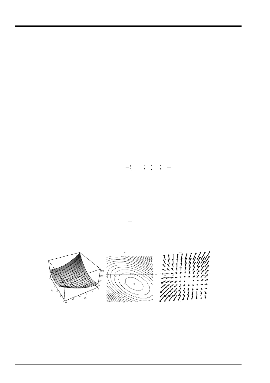
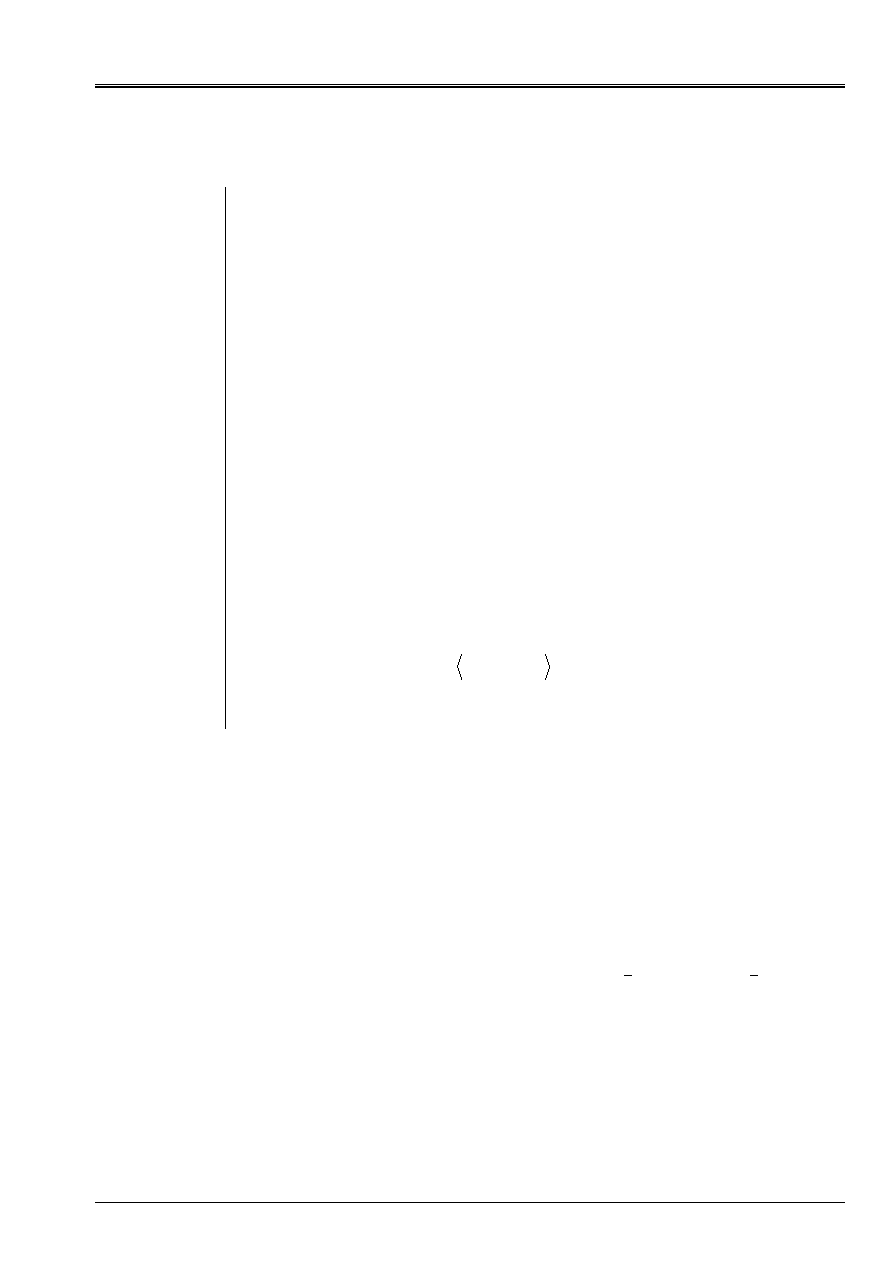
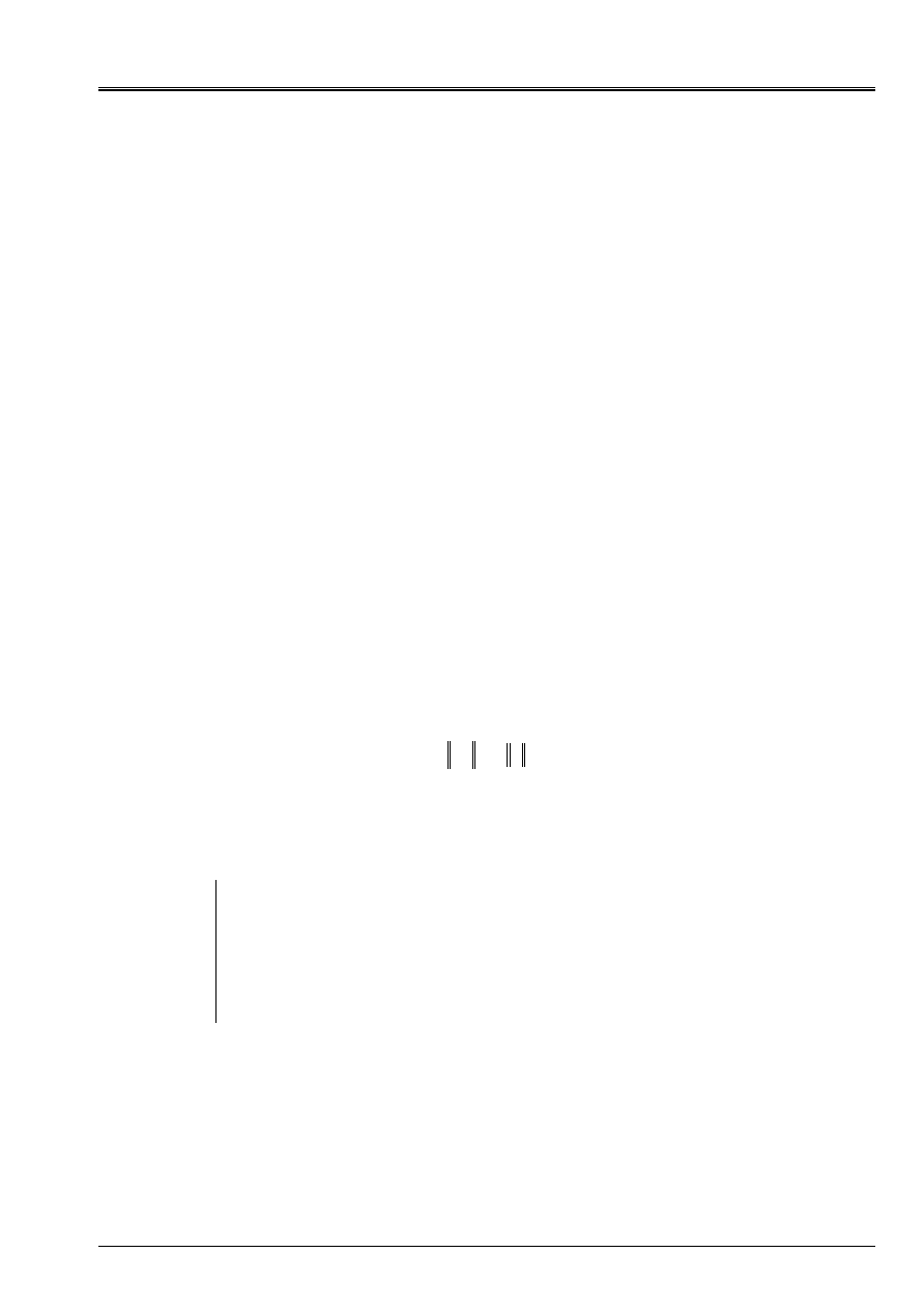
Appear 2.1-a: Example of

quadratic in N=2 dimensions with

and

graph (A), datum lines (b) and vectors gradient (c).

The spectrum of the operator is

(

) = (7;[1,2]

) and (

) = (2;[- 2,1]

(A)

(b)

(c)

Code_Aster

Version

6.4

Titrate:

Linear Solvor of combined gradient type

Date

17/02/04

Author (S):

O. BOITEAU, J.P. GREGOIRE, J. PELLET

Key

R6.01.02-B

Page

7/44

Manual of Reference

R6.01 booklet: Iterative methods

HI-23/03/001/A

This very important result in practice is based entirely on this famous definite-positivity property
a little “éthérée” the matrix of work. On a problem with two dimensions (

NR = 2

!) one can of

to make a limpid representation (cf [Figure 2.1-a]): the form paraboloid which focuses the single minimum
at the item [2, - 2]

of null slope.

· Minimization of the standard in energy of the error

()

, more speaking for

mechanics,

()

() ()

()

(

) ()

()

min

Arg

with

éq

2.1-4

From a mathematical point of view, it is anything else only one matric standard (licit since

SPD). One often prefers to express it via a residue

()

éq

2.1-5

Note:

· The perimeter of use of the combined gradient can in fact of extending to any operator,

not inevitably symmetrical or definite positive and even square! With this intention one defines
solution of

)

as being that, within the meaning of least squares, of the problem of

minimization

()

min

Arg

éq

2.1-6

By derivation one leads to the equations known as “normal” which the operator is square,
symmetrical and positive

()

éq

2.1-7

One can thus apply a GC to him or one steepest-descent without too much of tie up.

· The solution of the problem

)

is with the intersection of

hyperplanes of dimension

N-1

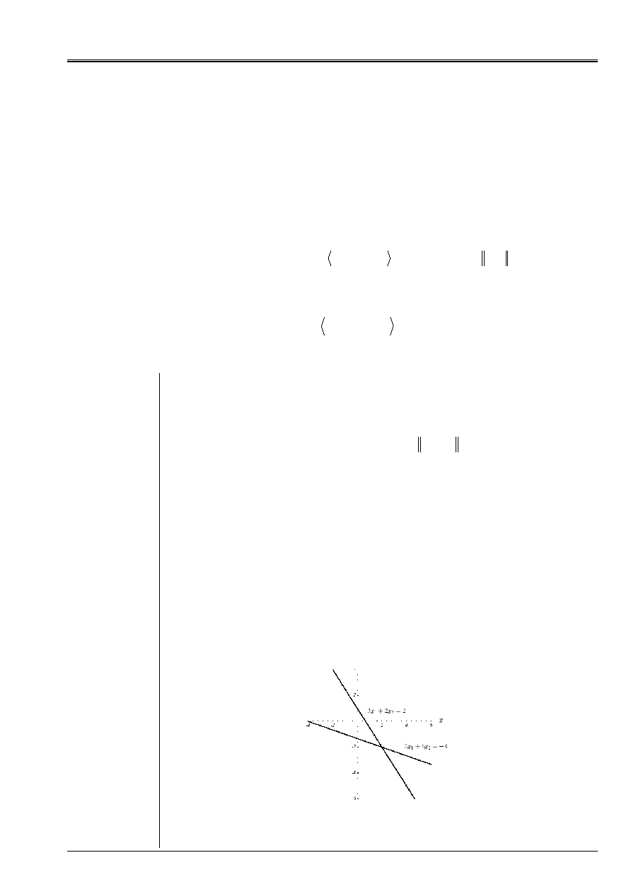
For example, in the case of [Figure 2.1-a], it is expressed trivialement in form
intersections of straight lines:

éq

2.1-8

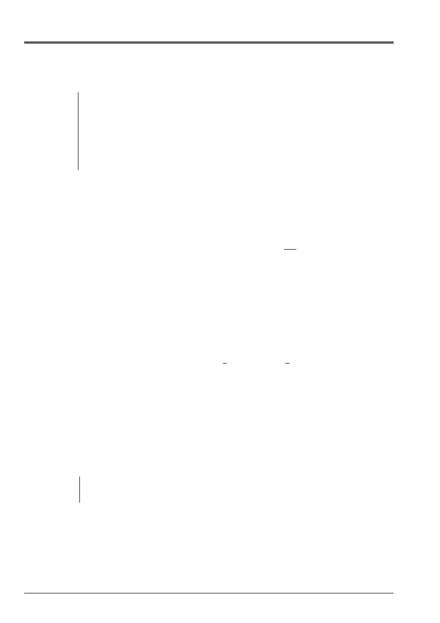
Appear 2.1-b: Resolution of the n°1 example by intersection of straight lines.

Code_Aster

Version

6.4

Titrate:

Linear Solvor of combined gradient type

Date

17/02/04

Author (S):

O. BOITEAU, J.P. GREGOIRE, J. PELLET

Key

R6.01.02-B

Page

8/44

Manual of Reference

R6.01 booklet: Iterative methods

HI-23/03/001/A

The methods of the gradient type dissociate this philosophy, they are registered
naturally within the framework of minimization of a quadratic functional calculus, in
which they were developed and intuitively included/understood.

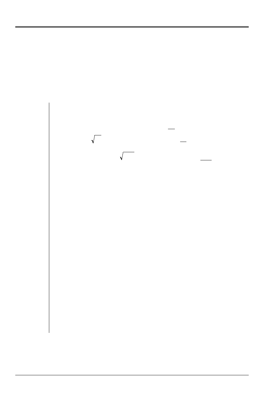
· When the matrix is not definite positive (cf [Figure 2.1-a] (A)), three cases of figures

present themselves: it is definite negative ((b), that does not pose a problem, one works
with

to minimize instead of maximizing), singular ((c), the whole of

solutions, if there exists, is a hyperplane) or unspecified ((D), it is about a problem of
not saddle on which the methods of the descent type or combined gradient stumble).

Appear 2.1-c: Form

according to the properties of

· The error

(v)

who expresses the distance from the intermediate solution to the exact solution and

the residue

(v),

the error which this intermediate solution implies on the resolution of

linear system, are bound by the relation

()

éq

2.1-9

More important, this residue is the opposite of the gradient of the functional calculus

()

éq

2.1-10

It is thus necessary to interpret the residues like potential directions of descent
allowing to decrease the values of

(they are orthogonal with the lines

isovaleurs cf [Figure 2.1-a]). These basic recalls proves to be useful thereafter.

Code_Aster

Version

6.4

Titrate:

Linear Solvor of combined gradient type

Date

17/02/04

Author (S):

O. BOITEAU, J.P. GREGOIRE, J. PELLET

Key

R6.01.02-B

Page

9/44

Manual of Reference

R6.01 booklet: Iterative methods

HI-23/03/001/A

2.2 Steepest

Descent

Principle

This last remark precedes the philosophy of the method known as “of the strongest slope”, more
known under its Anglo-Saxon denomination of “Steepest Descent”: one builds the continuation of reiterated

according to the direction whereby

decrease more, at least locally, i.e.

with

()

and

. With

ème

iteration, one thus will seek to build

i+1

such as:

éq 2.2-1

and

éq 2.2-2

Thanks to this formulation, one thus transformed a quadratic problem of minimization of size

(in

and

) in a unidimensional minimization (in

and

)

[

]

()

(

)

Arg

min

with

that

such

To find

éq

2.2-3

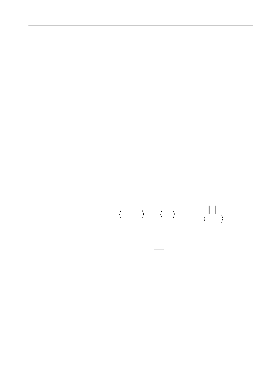
The following figures illustrate the operation of this procedure on the n°1 example: on the basis of
not

= [- 2, - 2]

(cf (A)) the optimal parameter of descent is sought,

, according to the line moreover

great slope

; what amounts seeking a point pertaining to the intersection of a vertical plane and

of a paraboloid (b), meant by the parabola (c). Trivialement this point cancels the derivative of
parabola (D)

()

éq 2.2-4

This orthogonality between two successive residues (i.e successive gradients) produced a routing
characteristic, known as in “zigzag”, towards the solution (E). Thus, in the case of a badly conditioned system
producing narrow and lengthened ellipses (the conditioning of operator SPD

is written like

the report/ratio of its extreme eigenvalues

()

min

max

who are themselves proportional to

axes of the ellipses. From where a direct and visual link between bad matric conditioning and narrow valley
and tortuous where minimization is abused), the iteration count necessary can be considerable
(cf [Figure 2.2-b] (b)).

Code_Aster

Version

6.4

Titrate:

Linear Solvor of combined gradient type

Date

17/02/04

Author (S):

O. BOITEAU, J.P. GREGOIRE, J. PELLET

Key

R6.01.02-B

Page

10/44

Manual of Reference

R6.01 booklet: Iterative methods

HI-23/03/001/A

Be reproduced 2.2-a Illustration of Steepest Descent on the n°1 example: direction of initial descent (A),

intersection of surfaces (b), corresponding parabola (c), vectors gradient and their projection

along the direction of initial descent (D) and total process until convergence (E).

Algorithm

From where unfolding

example)

(by

via

stop

Test

reiterated)

(new

descent)

optimal

(parameter

residue)

(new

Loop

given

tion

Initialized

)

(

)

(

)

(

)

(

Algorithm 1: Steepest Descent.

To save a product matrix-vector it is preferable to substitute at the stage (1), the update
residue following

éq

2.2-5

However, so avoiding inopportune accumulations of flares, one recomputes it periodically
residue with the initial formula (1).

has

Code_Aster

Version

6.4

Titrate:

Linear Solvor of combined gradient type

Date

17/02/04

Author (S):

O. BOITEAU, J.P. GREGOIRE, J. PELLET

Key

R6.01.02-B

Page

11/44

Manual of Reference

R6.01 booklet: Iterative methods

HI-23/03/001/A

Elements of theory

One shows that this algorithm converges, for any starting point

, at the speed (definite positivity

of the operator ensures us of the “good nature” of the parameter

. It is well an attenuation factor

because

)

()

with

éq

2.2-6

By developing the error on the basis of clean mode

(

;

)

matrix

()

éq 2.2-7

the attenuation factor of the error in energy becomes

(

)

(

) (

)

éq

2.2-8

In [éq 2.2-8], the fact that components

are squared ensures the priority ousting of the values

clean dominant. One finds here one of the characteristics of the modal methods of Krylov type
(Lanczos, Arnoldi cf [bib2] [§5] [§6]) which privileges the extreme clean modes. For this reason,
Steepest Descent and the combined gradient known as “coarse” is compared to the iterative solveurs
conventional (Jacobi, Gauss-Seidel, SOR…) more “smooth” bus eliminating without discrimination all them
components with each iteration.
Finally, thanks to the inequality of Kantorovitch (some is

stamp SPD and

vector not no one:

()

(

)

) one improves the legibility of the factor largely

of attenuation [éq 2.2-6]. At the end of

iterations, in the worst case, the decrease is expressed in the form

()

éq

2.2-9

It ensures linear convergence (i.e.

()

lim

. The rate

of asymptotic convergence

report/ratio of Kantorovitch is called) process in a number

iterations proportional to the conditioning of the operator. Thus, to obtain

()

(

)

small

éq 2.2-10

Code_Aster

Version

6.4

Titrate:

Linear Solvor of combined gradient type

Date

17/02/04

Author (S):

O. BOITEAU, J.P. GREGOIRE, J. PELLET

Key

R6.01.02-B

Page

12/44

Manual of Reference

R6.01 booklet: Iterative methods

HI-23/03/001/A

one needs an iteration count about

()

éq 2.2-11

A badly conditioned problem will thus slow down the convergence of the process, which one had already
“visually” noted with the phenomenon of “narrow and tortuous valley”.

For better apprehending the implication of the spectrum of the operator and starting point in
unfolding of the algorithm, let us simplify the formula [éq 2.2-8] while placing itself in the commonplace case where

While noting

the matric conditioning of the operator and

the slope of the error with

ème

iteration (in the frame of reference of the two clean vectors), one obtains an expression more
readable of the attenuation factor of the error (cf [Figure 2.2-b])

(

)

(

) (

)

éq

2.2-12

As for the modal solveurs, one notes that the importance of the conditioning of the operator is
balanced by the choice of a good starting point: in spite of a bad conditioning, the cases (A) and (b)
are very different; In the first, the starting point generates almost a clean space of
the operator and one converge in two iterations, if not they are the “sempiternal zigzags”.

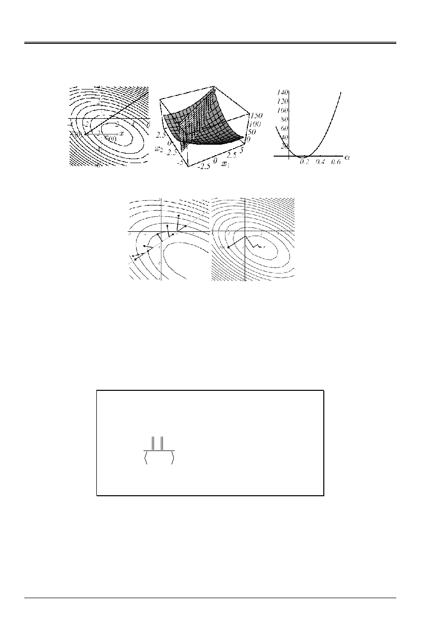
(E)

Be reproduced 2.2-b: Convergence of Steepest Descent on the n°1 example according to the values of

conditioning and of the starting point:

large and

small (A),

and

large (b),

and

small (c),

small and

large (D) and forms total

(

, µ

) (E).

Code_Aster

Version

6.4

Titrate:

Linear Solvor of combined gradient type

Date

17/02/04

Author (S):

O. BOITEAU, J.P. GREGOIRE, J. PELLET

Key

R6.01.02-B

Page

13/44

Manual of Reference

R6.01 booklet: Iterative methods

HI-23/03/001/A

Note:

· This method of the strongest slope was initiated by Cauchy (1847) and was given to the taste

day by Curry (1944). Within the framework of operators SPD, it is also sometimes
called method of the gradient with optimal parameter (cf [bib26] [§8.2.1]). In spite of its
weak properties of convergence, she knew her “hour of glory” to minimize
functions

quasi-unspecified, makes some only derivable. In this case of

appear more general, it then allows to reach only stationary points, with
better local minima.

· To avoid zigzag the proceeded various effects of acceleration were proposed

(cf Forsythe 1968, Luenberger 1973 or [bib28] [§2.3]) which has a speed of
convergence similar to that of the gradient combined but for a calculation complexity
quite higher. They thus fell gradually in disuse.
Let us note that alternatives of algorithm 1 were introduced to treat cases not
SPD: Iteration of the minimum residue and Steepest Descent with standard of the residue
(cf [bib35] [§5.3.2] [§5.3.3]).

· One finds through Steepest Descent a very widespread key concept in analysis

numerical: that of the resolution of a problem, by projection of reiterated on under
space approximating

, here

vect (R

)

, perpendicular to another under

space, here

:=K

. They are called, respectively, space of search or

of approximation and space of stress. For Steepest Descent, they are equal and
reduced to their simpler expression but we will see that for the combined gradient
they take the form of particular spaces, known as of Krylov.
Formally, with each iteration

algorithm, one seeks an increment thus

such as:

éq

2.2-13

This general framework constitutes the conditions of Petrov-Galerkin what is called
(cf [bib35] [§5]).

Complexity and occupation memory

The major part of the cost calculation of algorithm 1 lies in the update [éq 2.2-5] and, more
particularly, in the product matrix-vector

. In addition, it was already mentioned that its

convergence was acquired and took place in an iteration count proportional to complexity of
stamp (cf [éq 2.2-11]).
Its complexity is thus, if one takes account of the hollow character of the operator, about

()

(

)

where

is the average number of nonnull terms per line of

The discretization finite elements of the elliptic operators of the second command (resp. fourth command)
(case generally encountered in mechanics of the structures) implying conditionings
operators in

()

(

)

(resp.

()

(

)

), with

the dimension of space,

calculation complexity of Steepest Descent within this framework is written

(resp.

As regards the occupation memory, only the storage of the matrix of work is possibly
necessary (in the absolute, Steepest Descent as the GC requires only the knowledge of the action
matrix on an unspecified vector and not its storage in extenso. This facility can
to prove to be invaluable for very greedy applications in DDLs (CFD, electromagnetism…)) :

()

. In practice, the data-processing installation of hollow storage imposes the management of vectors

additional entireties: for example, for MORSE storage used in Code_Aster, vectors

indices of end of line and indices of columns of the nonnull elements of the profile. From where one
effective memory complexity of

()

realities and

(

)

entireties.

Code_Aster

Version

6.4

Titrate:

Linear Solvor of combined gradient type

Date

17/02/04

Author (S):

O. BOITEAU, J.P. GREGOIRE, J. PELLET

Key

R6.01.02-B

Page

14/44

Manual of Reference

R6.01 booklet: Iterative methods

HI-23/03/001/A

2.3

Method of “general” descent

Principle

A crucial stage of these methods is the choice of their direction of descent (per definition one

direction of descent (dd) with

ème

stage,

, checks:

()

) (dd). Even if the gradient of

functional calculus remains the main product about it, one can choose another version completely of it

that that

required for Steepest Descent. With

ème

iteration, one thus will seek to build

i+1

checking

éq 2.3-1

with

[

]

(

)

Arg

min

éq

2.3-2

It is of course only one generalization of Steepest Descent seen previously and it is shown that
its choices of the parameter of descent and its property of orthogonality spread

éq 2.3-3

From where the same effect “zigzag” during unfolding of the process and a convergence similar to
[éq 2.2-6] with an attenuation factor of the error undervalued by:

()

éq

2.3-4

This result one can then formulate two official reports:

· the conditioning of the operator intervenes directly on the attenuation factor and thus on

the speed of convergence,

· to ensure itself of convergence (sufficient condition) one needs, at the time of a given iteration, that

the direction of descent is not orthogonal with the residue.

The sufficient condition of this last item is of course checked for Steepest Descent (

) and it

a choice of direction of descent for the combined gradient will impose. To mitigate the problem
raised by the first point, we will see that it is possible to constitute an operator of work

whose conditioning is less. One speaks then about prepacking.

Code_Aster

Version

6.4

Titrate:

Linear Solvor of combined gradient type

Date

17/02/04

Author (S):

O. BOITEAU, J.P. GREGOIRE, J. PELLET

Key

R6.01.02-B

Page

15/44

Manual of Reference

R6.01 booklet: Iterative methods

HI-23/03/001/A

Always in the case of an operator SPD, course of a method of “general” descent
is thus written

)

(

)

(

)

(

)

(

)

(

)

(

Calculation

example)

(by

via

stop

Test

residue)

(new

reiterated)

(new

descent)

optimal

(parameter

Loop

given,

tion

Initialized

Algorithm 2: Method of descent in the case of a quadratic functional calculus.

This algorithm precedes already well that of the Gradient Combined (GC) which we will examine in the chapter
according to (cf algorithm 4). It shows well that the GC is only one method of descent applied in
the framework of quadratic functional calculuses and specific directions of descent. Finally, only
the stage (6) will be some packed.

Note:

· By successively posing like directions of descent the canonical vectors of

axes of co-ordinates of space with

dimensions (

), one obtains the method of

Gauss-Seidel.

· To avoid the overcost calculation of the stage of unidimensional minimization (2) (produced

matrix-vector) one can choose to fix the parameter of descent arbitrarily: it is
method of Richardson who converges as well as possible like Steepest Descent.

Complements

With a functional calculus

continue unspecified (cf [Figure 2.3-a] (A)), one exceeds the strict framework of

the linear inversion of system for that of unconstrained nonlinear continuous optimization (

then often called function objective cost or function). Two simplifications which had runs up to now
become illicit then:

· The reactualization of the residue

stage (4),

· The simplified calculation of the optimal parameter of descent

stage (2).

Their reasons to be being only to use all the assumptions of the problem to facilitate
unidimensional minimization [éq 2.3-2], one is then constrained to explicitly carry out this
linear search on a functional calculus chahutée with this time of multiple local minima.
Fortunately, there is a whole panoply of methods according to the degree of necessary information on
function cost

(quadratic interpolation, dichotomy on the values of the function, the gilded section,

regulate of Goldstein and Price…),

(dichotomy on the values of the derivative, regulates of Wolfe, Armijo…),

(Newton-Raphson…)

· …

Code_Aster

Version

6.4

Titrate:

Linear Solvor of combined gradient type

Date

17/02/04

Author (S):

O. BOITEAU, J.P. GREGOIRE, J. PELLET

Key

R6.01.02-B

Page

16/44

Manual of Reference

R6.01 booklet: Iterative methods

HI-23/03/001/A

As regards the search for descent, there too of many solutions are proposed in
literature (combined gradient nonlinear, quasi-Newton, Newton, Levenberg-Marquardt (these two
last methods are used by Code_Aster: the first in the nonlinear operators
(STAT/DYNA/THER_NON_LINE), the second in the macro one of retiming (MACR_RECAL)) …). Of

long date, methods known as of nonlinear combined gradient (Fletcher-Reeves (FR) 1964 and
Polak-Ribière (PR) 1971) proved to be interesting: they converge superlinéairement towards one
local minimum at a reduced cost calculation and overall dimension memory (cf [Figures 2.3-a]).
They lead to the choice of an additional parameter

who manages the linear combination between

directions of descent

()

with

éq 2.3-5

Appear 2.3-a: Example of

nonconvex in

=2: graph (A), convergence with

a nonlinear GC of type Fletcher-Reeves (b), plan of cut

the first unidimensional search (c).

has

Code_Aster

Version

6.4

Titrate:

Linear Solvor of combined gradient type

Date

17/02/04

Author (S):

O. BOITEAU, J.P. GREGOIRE, J. PELLET

Key

R6.01.02-B

Page

17/44

Manual of Reference

R6.01 booklet: Iterative methods

HI-23/03/001/A

From where the algorithm, while naming

opposite of the gradient and either the residue (which does not take place any more to be here),

[

]

(

)

()

dd)

(news

conjugaiso

(parameter

example)

(by

via

stop

Test

gradient)

(new

reiterated)

(new

descent)

(parameter

To find

Loop

given,

tion

Initialized

Arg

)

(

)

(

)

(

)

(

)

(

min

)

(

Algorithm 3: Methods of the nonlinear combined gradient (FR and PR).

Nonlinear designation combined gradient is rather here synonymous with “nonconvex”: there is no more
of dependence the problem of minimization enters

)

and a linear system

)

. With the sight of

algorithm 4, the great similarities with the GC consequently appear completely clear. Within the framework
to a quadratic function cost of type [éq 2.1-2b], it is just enough to substitute at the stage (1)
updating of the residue and the calculation of the optimal parameter of descent. The GC is only one method of
Fletcher-Reeves applied to the case of a convex quadratic functional calculus.

Now that we started well the link between the methods of descent, the combined gradient
with the linear direction solvor SPD and his version, sight of the end of the spyglass optimization continues not
linear, we go (finally!) to pass to sharp from the subject and to argue the choice of a direction of descent
type [éq 2.3-5] for the standard GC.
For more information on the methods of the descent type, the reader will be able to refer to excellent
works of optimization (in French language) of Mr. Minoux [bib28], J.C. Culioli [bib11] or
J.F. Bonnans et al. [bib5].

Code_Aster

Version

6.4

Titrate:

Linear Solvor of combined gradient type

Date

17/02/04

Author (S):

O. BOITEAU, J.P. GREGOIRE, J. PELLET

Key

R6.01.02-B

Page

18/44

Manual of Reference

R6.01 booklet: Iterative methods

HI-23/03/001/A

The combined gradient (GC)

3.1 Description

general

Principle

Now that the bases are set up we will be able to approach the algorithm of the Gradient
Combined (GC) itself. It belongs to a subset of methods of descent which
gather the methods known as “of combined directions” (the methods of Fletcher-Reeves and of
Polak-Ribière (cf [§2.3]) form also part of this family of methods). Those recommend
to build directions of descents gradually

… linearly independent of

manner to avoid the zigzags of the method of conventional descent.
Which linear combination then to recommend to build, at the stage

, new direction of

descent? Knowing of course that it must take account of two crucial information: the value of
gradient

and those of the preceding directions

éq

3.1-1

The easy way consists in choosing a vectorial independence of type

- orthogonality (like the operator

of work is SPD, it defines well a scalar product via which two vectors can be orthogonal)
(cf [Figure 3.1-a])

()

= 0

éq

3.1-2

also called conjugation, from where the designation of the algorithm. It makes it possible to propagate of close relation in
near orthogonality and thus to calculate only one coefficient of Gram-Schmidt to each iteration.
From where a gain in calculation complexity and very appreciable memory.

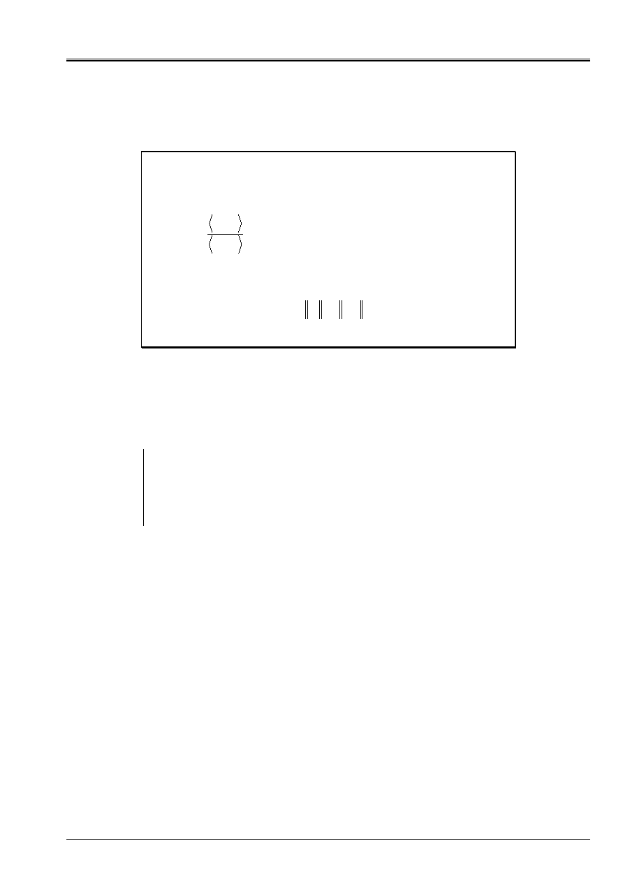
Appear 3.1-a: Example of pairs of vectors

- orthogonal in 2D: conditioning

unspecified (A), perfect conditioning (i.e equal to the unit) = usual orthogonality (b).

One can thus be satisfied with a linear combination of the type

éq 3.1-3

And this, more especially as it checks the sufficient condition [éq 2.3-4] and that because of orthogonality
[|éq 2.3-3b], the unidimensional search [éq 2.3-2] which follows takes place in an optimal space: the plan
formed by the two orthogonal directions

, D

i-1

)

It thus remains to determine the optimal value of the proportionality factor

. In the GC this choice

take place so as to maximize the attenuation factor of [éq 2.3-4], i.e. the term

éq

3.1-4

Code_Aster

Version

6.4

Titrate:

Linear Solvor of combined gradient type

Date

17/02/04

Author (S):

O. BOITEAU, J.P. GREGOIRE, J. PELLET

Key

R6.01.02-B

Page

19/44

Manual of Reference

R6.01 booklet: Iterative methods

HI-23/03/001/A

It leads to the expression

éq

3.1-5

and the same property of orthogonality of the successive residues as for Steepest Descent induces (but
without the zigzags!)

éq

3.1-6

A condition “residue-dd is added”

éq

3.1-7

who forces to initialize the process via

Algorithm

In short, by recapitulating the relations [éq 2.2-5], [éq 2.3-1], [éq 2.3-3] and [éq 3.1-3], [éq 3.1-5], [éq 3.1-7] it
occurs the conventional algorithm

dd)

(news

)

optimal

conjugaiso

parameter

(

)

example

(

via

stop

Test

)

residue

new

(

)

reiterated

new

(

)

descent

optimal

parameter

(

Loop

given,

tion

Initialized

)

(

)

(

)

(

)

(

)

(

)

(

)

(

Algorithm 4: Standard combined gradient (GC).

Code_Aster

Version

6.4

Titrate:

Linear Solvor of combined gradient type

Date

17/02/04

Author (S):

O. BOITEAU, J.P. GREGOIRE, J. PELLET

Key

R6.01.02-B

Page

20/44

Manual of Reference

R6.01 booklet: Iterative methods

HI-23/03/001/A

On the n°1 example, the “supremacy” of the GC compared to Steepest Descent is manifest
(cf [Figures 3.1-b]) and is explained by the results of convergence [éq 2.2-9] and [éq 3.2-9]. In
two cases, the same points starting and the same criteria of stop were selected:

= [- 2, - 2]

and

Appear 3.1-b: Convergences compared of Steepest Descent (A)

and of the GC (b) on the n°1 example.

Note:

· This method of the GC was developed independently by Mr. R. Hestenes (1951) and

E.Stiefel (1952) of the “National Office off Standard” of Washington D.C. (seedbed of
numericians with also C.Lanczos). First theoretical results of convergence
are due to work of S. Kaniel (1966) and H.A. Van der Vorst (1986) and it has
really popularized for the resolution of large hollow systems by J.K.Reid
(1971). The interested reader will find a history commented on and a bibliography
exhaustive on the subject in papers of G.H. Golub, H.A Van der Vorst and Y. Saad
[bib15], [bib16], [bib36].

· For the small history, extremely of its very broad dissemination in the industrial world and

academic, and, of his many alternatives, the GC was classified in third position
of the “Top10” of the best algorithms of the XX

century [bib10]. Just behind

methods of Monte Carlo and the simplex but in front of the algorithm

, them

transforms of Fourier and the solveurs multipôles!

· One finds traces in the codes of EDF R & D of the GC as of the beginning of the Eighties with

the first work on the subject of J.P. Gregoire [bib18] [bib21]. Since it is
spread, with an unequal happiness, in many fields, _ N3S,
Code_Saturne, LADYBIRD, Code_Aster, TRIFOU, ESTET, TELEMAC _, and it was
much optimized, vectorized and paralleled [bib19], [bib20], [bib22], [bib23].

Note:

Being very depend on the conditioning of the matrices generated by these
fields of physics, it is generally more used in mechanics of
fluids or in electromagnetism that into thermomechanical of the structures.
From where supremacy, in this last field of activities, of the direct solveurs…
Code_Aster with its multifrontale [bib33] not escaping the rule. One y
cumulate often strong heterogeneities of material, loading and size
of mesh, non-linearities and junctions elements isoparametric/elements
structural which gangrènent dramatically this conditioning [bib31],
[bib13].

· With the test of stop on the standard of the residue, theoretically licit but in practice sometimes

difficult to gauge, one often prefers a criterion of adimensional stop, such as the residue

relative to

ème

iteration:

(cf [§5.2]).

has

Code_Aster

Version

6.4

Titrate:

Linear Solvor of combined gradient type

Date

17/02/04

Author (S):

O. BOITEAU, J.P. GREGOIRE, J. PELLET

Key

R6.01.02-B

Page

21/44

Manual of Reference

R6.01 booklet: Iterative methods

HI-23/03/001/A

3.2

Elements of theory

Space of Krylov

By carrying out a second analysis of Petrov-Galerkin already evoked for Steepest Descent, one can synthesize
in a sentence the action of the GC. It carries out successive orthogonal projections on the space of
Krylov

(

)

(

)

vect

where

is the initial residue

: with

ème

iteration

(

)

, R

= L

. One solves the linear system (

) by seeking an approximate solution

in the subspace refines (space of search for dimension

NR)

(

)

, R

With

éq

3.2-1

while imposing the stress of orthogonality (space of the stresses of dimension

NR)

(

)

éq

3.2-2

This space of Krylov to the good property to facilitate the approximation of the solution, at the end of

iterations, in the form

()

éq

3.2-3

where

M-1

is a certain matric polynomial of command

M-1

. Indeed, it is shown that the residues and them

directions of descent generate this space

(

)

(

)

(

)

(

)

vect

éq

3.2-4

while allowing the approached solution,

, to minimize the standard in energy on all space

closely connected

With

With

éq

3.2-5

This gasket result with the property [éq 3.2-4b] illustrates all the optimality of the GC: contrary to the methods
of descent, the minimum of energy is not carried out successively for each direction of
descent, but jointly for all the directions of descent already obtained.

Note:

One distinguishes a large variety from methods of projection on spaces of the Krylov type,
called more prosaically “methods of Krylov”. To solve systems
linear [bib35], [bib27] (GC, GMRES, FOM/IOM/DOM, GCR, ORTHODIR/MIN…) and/or of
modal problems [bib2], [bib39] (Lanczos, Arnoldi…). They differ by the choice from their
space of stress and by that of the prepacking applied to the initial operator for
to constitute that of work, knowing that different establishments lead to
algorithms radically distinct (vectorial version or per blocks, tools
of orthonormalisation…).

Code_Aster

Version

6.4

Titrate:

Linear Solvor of combined gradient type

Date

17/02/04

Author (S):

O. BOITEAU, J.P. GREGOIRE, J. PELLET

Key

R6.01.02-B

Page

22/44

Manual of Reference

R6.01 booklet: Iterative methods

HI-23/03/001/A

Orthogonality

As one already announced, the directions of descents are

- orthogonal between them. Moreover, it

choice of the optimal parameter of descent (cf [éq 2.2-4], [éq 2.3-3a] or stage (2)) impose, of close relation in
near, orthogonalities

éq

3.2-6

One thus notes a small approximation in the name of the GC, because the gradients are not
combined (cf [éq 3.2-6b]) and the directions combined do not comprise only gradients
(cf [éq 3.1-3]). But “let us not haggle” not, the indicated products are nevertheless there!

With the exit of

iterations, two cases of figures arise:

· That is to say the residue is null

convergence.

· Either it is orthogonal with

preceding directions of descent which constitute a base of

the finished space of approximation

(as they are linearly independent). From where

necessarily

convergence.

It would thus seem that the GC is a direct method which converges in at the maximum

iterations, it is

less what one believed before testing it on practical cases! Because what remains true in theory, in
arithmetic exact, is put at evil by arithmetic finished computers. Gradually,
in particular because of the round-off errors, the directions of descent lose their beautiful properties of
conjugation and minimization leaves necessary space.
Known as differently, one solves an approximate problem which is not completely any more the projection desired of
initial problem. The method (theoretically) direct revealed its true nature! It is iterative and thus
subjected, in practice, with many risks (conditioning, starting point, tests of stop, precision
orthogonality…).

To cure it, one can force during the construction of the new direction of descent
(cf algorithm 4, stage (7)), a phase of reorthogonalisation. This very widespread practice in
analyze modal (cf [bib2] [§5.3.1] and appendix 2) and in decomposition of field (cf [bib4] [§5.2.6])
can decline itself under various alternatives: total, partial, selective reorthogonalisation… via all
a panoply of procedures of orthogonalization: GS, GSM, IGSM, Househölder, Givens… For
methods of the Krylov type, in order to spare the occupation memory and by preoccupations with a robustness, one
recommend réorthogonaliser systematically only compared to the first directions which
generate the subspace invariant associated the with greatest eigenvalues (in processing with
signal, this space would define what one call the coherent structure of the field of solution displacement,
i.e. its substantial marrow).
These réorthogonalisations require the storage of

orth

first vectors

(

)

orth

and of

their product by the operator of work

(

)

orth

= Kd

. Formally, it is thus about

to substitute at the two last stages of the algorithm following calculation

(

)

ized)

orthogonal

(news

orth

max

éq

3.2-7

Through the various numerical experiments which were undertaken (cf in particular work of
J.P. Gregoire and [bib3]), it seems that this reorthogonalisation is not always effective. Its
overcost due mainly to the new products matrix-vector

(and with their storage) is not

always compensated by the gain in iteration count total. Contrary to what is
generally observed in decomposition of field (iterative method of primal Schur and FETI) where
installation of this process is recommended. It is true that it intervenes then on a problem
of interface much smaller and conditioned better than the total problem.

Code_Aster

Version

6.4

Titrate:

Linear Solvor of combined gradient type

Date

17/02/04

Author (S):

O. BOITEAU, J.P. GREGOIRE, J. PELLET

Key

R6.01.02-B

Page

23/44

Manual of Reference

R6.01 booklet: Iterative methods

HI-23/03/001/A

Convergence

Because of particular structure of the space of approximation [éq 3.2-3] and property of
minimization on this space of the approximate solution

(cf [éq 3.2-5]), one obtains an estimate of

the speed of convergence of the GC

() () ()

()

(

)

max

with

éq

3.2-8

where one notes

(

;

)

clean modes of the matrix

and

M-1

an unspecified polynomial of degree with

more

. Famous polynomials of Tchebycheff, via their good properties of increase in

the space of the polynomials, make it possible to improve the legibility of this attenuation factor

At the end of

iterations, in the worst case, the decrease is expressed then in the form

()

éq

3.2-9

It ensures convergence superlinéaire (i.e.

()

lim

) of the process in one

iteration count proportional to the square root of the conditioning of the operator. Thus, for
to obtain

()

(

)

small

éq

3.2-10

one needs an iteration count about

()

éq 3.2-11

Obviously as we noticed many times, a badly conditioned problem will slow down
convergence of the process. But this deceleration will be less notable for the GC than for
Steepest Descent (cf [Figures 3.2-a]). And in any event, the total convergence of the first will be
better.

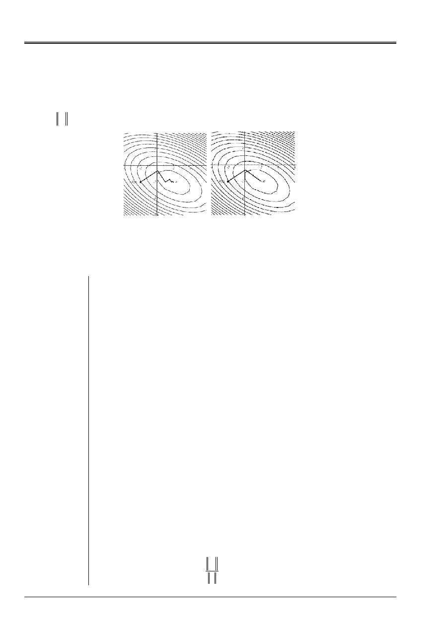
Appear 3.2-a: Convergences compared of Steepest Descent (A)
and of the GC (b) (with the factor ½ near) according to conditioning

(A)

(b)

Code_Aster

Version

6.4

Titrate:

Linear Solvor of combined gradient type

Date

17/02/04

Author (S):

O. BOITEAU, J.P. GREGOIRE, J. PELLET

Key

R6.01.02-B

Page

24/44

Manual of Reference

R6.01 booklet: Iterative methods

HI-23/03/001/A

Note:

· In practice, benefitting from particular circumstances, _ better starting point and/or

advantageous spectral distribution _, the convergence of the GC can be much better than
what lets hope [éq 3.2-9]. Methods of Krylov tending to flush out
firstly extreme eigenvalues, the “effective conditioning” of the operator
of work is some improved.

· On the other hand, certain iterations of Steepest Descent can get the best

decrease of the residue that same iterations of the GC. Thus, the first iteration of
GC is identical to that of Steepest-Descent and thus with a rate of convergence
equal.

Complexity and occupation memory

As for Steepest Descent, the major part of the cost calculation of this algorithm lies in
the stage (1), the product matrix-vector. Its complexity is about

(

)

kcN

where

is the number

means of nonnull terms per line of

and

the iteration count necessary to convergence. For

to be much more effective than simple Cholesky (of complexity

) it is thus necessary:

· To take well into account the hollow character of the matrices resulting from the discretizations elements

stop (MORSE storage, produced matrix-vector optimized adhoc):

· Préconditionner the operator of work:

One already pointed out that for an operator SPD his theoretical convergence occurs in, at most,

iterations and proportionally with the root of conditioning (cf [éq 3.2-11]). In practice, for

large badly conditioned systems (as it is often the case in mechanics of the structures), it
can be very slow to appear (cf phenomenon of Lanczos of the following paragraph).
Taking into account conditionings of operators generally noted in mechanics
structures and recalled for the study of complexity of Steepest Descent, which one takes them again

notations, calculation complexity of the GC is written

1
D

(resp.

As regards the occupation memory, as for Steepest Descent, only the storage of
stamp work is possibly necessary:

()

. In practice, the data-processing installation of

hollow storage imposes the management of additional vectors of entireties: for example for
storage MORSE used in Code_Aster, vectors of the indices of end of line and the indices of
columns of the elements of the profile. From where effective a memory complexity of

()

realities and

(

)

entireties.

Note:

These considerations on the overall dimension memory do not take into account the problems
of storage of a possible preconditionnor and workspace which its construction can
temporarily to mobilize.

Code_Aster

Version

6.4

Titrate:

Linear Solvor of combined gradient type

Date

17/02/04

Author (S):

O. BOITEAU, J.P. GREGOIRE, J. PELLET

Key

R6.01.02-B

Page

25/44

Manual of Reference

R6.01 booklet: Iterative methods

HI-23/03/001/A

3.3 Complements

Equivalence with the method of Lanczos

In “triturating” the property of orthogonality of the residue with any vector of the space of Krylov
(cf [éq 3.2-2]), it is shown that them

iterations of the GC lead to the construction of one factorized of

Lanczos of the same command (cf [bib2] [§5.2])

éq

3.3-1

while noting:

the specific “residue” of this factorization,

ième

vector of the canonical base,

the vectors residues standardized with the unit, called for the occasion vectors of

Lanczos,

the orthogonal matrix which they constitute.

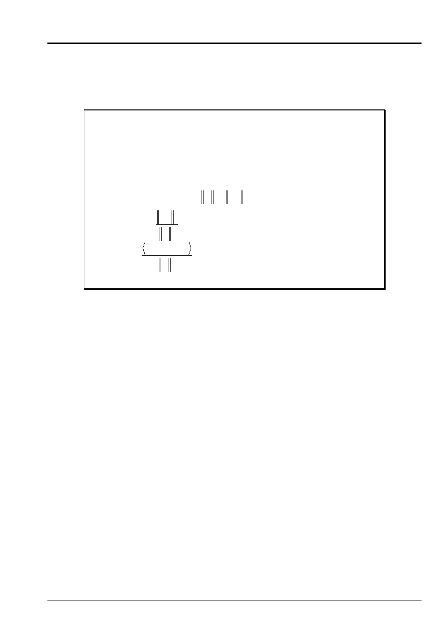
Appear 3.3-a: Factorization of Lanczos induced by the GC.

The matrix of Rayleigh which expresses the orthogonal projection of

on the space of Krylov

(

)

takes the canonical form then

…

éq

3.3-2

Code_Aster

Version

6.4

Titrate:

Linear Solvor of combined gradient type

Date

17/02/04

Author (S):

O. BOITEAU, J.P. GREGOIRE, J. PELLET

Key

R6.01.02-B

Page

26/44

Manual of Reference

R6.01 booklet: Iterative methods

HI-23/03/001/A

Almost without additional calculation, the GC thus provides the approximation of Rayleigh of the operator of
work in a form sympathetic nerve, _ symmetrical square matrix tridiagonale of flexible size _,
it will be easy to deduce the spectrum (via, for example, robust

cf [bib2] appendix 2)).

At the end of a linear inversion of system led by a simple GC one thus can, with less expenses,
to know, in addition to the sought solution, an approximation of the spectrum of the matrix and thus of
its conditioning [bib24]. This functionality should be inserted soon in Code_Aster of
manner to control the level of prepacking.

Note:

· The operator of work being SPD, his matrix of Rayleigh inherits this property and one

its decomposition obtains directly

()

with

…

and

éq 3.3-3

Method of Lanczos not calculating these intermediate terms

and

, but

directly the tridiagonaux terms, it does not have access to this information. On the other hand,
it can take into account symmetrical matrices not necessarily definite
positive.

· Therefore, that it is a question of reversing a linear system or of determining part of sound

spectrum, these methods of Krylov function on the same principle: to determine
gradually vectors of bases generating the space of projection into same
time that the result of this projection. In the GC as in Lanczos, one évertue
to make the this projection most robust (orthogonality of the basic vectors), more
reduced (size of projection = iteration count) and simplest possible (projection
orthogonal). For the modal solvor, another stress is juxtaposed: to approximate it
better possible the spectrum of the operator of work by that of the matrix of Rayleigh.
In nonsymmetrical, one speaks about either orthogonal but oblique projection and them
bringings together is carried out then between GMRES and Arnoldi [bib35].

· Into arithmetic exact, at the end of

iterations, one completely determined all it

spectrum of the operator. In practice, problems of flares and orthogonalization us
in prevent. But, if one is sufficiently patient (

NR!

), one is nevertheless

able to detect all the spectrum: it is what is called the phenomenon of Lanczos
(cf [bib2] [§5.3.1], [§5.3.3] or [bib39]).

Note:

Paradoxically the loss of orthogonality is especially ascribable with convergence
of a clean mode more than to the round-off errors! This analysis due to CC.Paige
(1980) attests that as soon as a clean mode is captured it the layout disturbs
orthogonal of the vectors of Lanczos (in the case which worries us, them
residues and directions of descent). Into modal, digital processing of it
parasitic phenomenon was the subject of many palliative developments. For
what is GC, it must attach the effectiveness of the methods of reorthogonalisation
directions of descent evoked previously.

Code_Aster

Version

6.4

Titrate:

Linear Solvor of combined gradient type

Date

17/02/04

Author (S):

O. BOITEAU, J.P. GREGOIRE, J. PELLET

Key

R6.01.02-B

Page

27/44

Manual of Reference

R6.01 booklet: Iterative methods

HI-23/03/001/A

Encased Solveurs

As one already pointed out, the linear solveurs are often hidden with deepest of others
algorithms, and in particular, of the nonlinear solveurs of Newton type. It is for Code_Aster them
cases of application most frequently used: operators STAT_NON_LINE, DYNA_NON_LINE and
THER_NON_LINE.

In such a configuration, a linear solvor such as the CG can fire his pin from the play (by report/ratio
with a direct solvor). Its iterative character proves to be useful to make evolve/move the test of stop of the algorithm
(cf stage (5) algorithm 4) according to the relative error of the nonlinear solvor who encapsulates it: it is
the problems encased solveurs (one also speaks about relieving) [bib12], [bib17], [bib8], [bib9] of which it
CERFACS is the “spearhead” in France.
By slackening at the convenient period the necessary precision on the cancellation of the residue (for example strategy
in the case modal method of Krylov type + GC [bib8]) or, on the contrary by hardening it
(resp. modal method of power type + Gauss-Seidel + GC [bib9]), one can thus gain in
calculation complexity on the GC without modifying the convergence of the total process. It is of course necessary to put
at the point of the simple and inexpensive criteria so that the gain is substantial. This functionality
should be inserted soon in Code_Aster (internal and automatic piloting of the value
RESI_RELA).

Note:

Certain authors also put the question about sequence of these
algorithms: “Newton GC” or “GC Newton”? If from a data-processing point of view and
conceptual, the question is quickly distinct: one prefers the first solution, more readable, more
flexible and which does not disturb existing it, from a numerical and algorithmic point of view, it
sharing is more moderate. That can depend on the “technical tripailles” deployed by
non-linear solvor (tangent matrix, unidimensional minimization…) and of the deployed GC
(preconditionnor). Nevertheless, it seems that the natural command, “Newton GC”, is more
effective and most evolutionary.

Parallelism

The GC as much of iterative solveurs lends itself well to parallelism. It is scalable, i.e.
that if a calculation with

ddls functions on

processors, its during with

must function on

main elementary operations which constitutes it (produced matrix-vector and scalar product)
break up effectively between various processors, only the parallelization of the preconditionnor
(often based on a direct solvor) can prove to be hazardous (problems often called:
“parallel preconditioning”).
Thus on the CRAY machine, J.P. Gregoire adapted and paralleled, in memory shared [bib20] and in
distributed memory [bib23], an algorithm of packaged combined the gradient type. Four types
operations are carried out jointly: elementary vectorial operations, products
scalars, the products matrix-vector and the construction of the preconditionnor (diagonal). Problems
of “parallel preconditioning” which was solved only for the diagonal preconditionnor, do not have
unfortunately not allowed the bearing of these models in the official version of Code_Aster.

We besides now will tackle the thorny question of prepacking for the GC. It
will become the Packaged Combined Gradient then: GCPC.

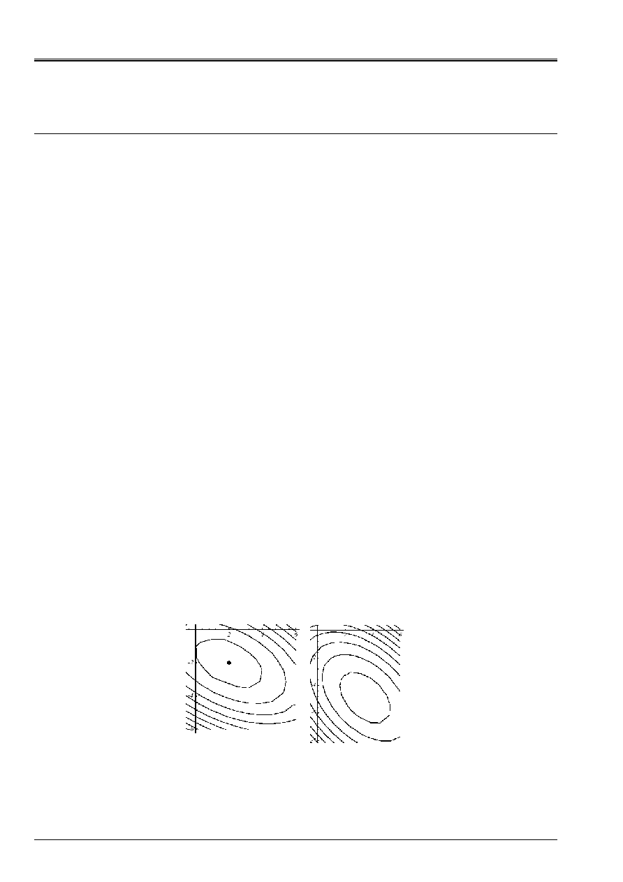
Code_Aster

Version

6.4

Titrate:

Linear Solvor of combined gradient type

Date

17/02/04

Author (S):

O. BOITEAU, J.P. GREGOIRE, J. PELLET

Key

R6.01.02-B

Page

28/44

Manual of Reference

R6.01 booklet: Iterative methods

HI-23/03/001/A

The packaged combined gradient (GCPC)

4.1 Description

general

Principle

Like one could note it (and to hammer it!) in the preceding paragraphs, the speed of
convergence of the methods of descent, and in particular that of the combined gradient, depends on
conditioning of the matrix

()

. More it is close to its value floor, 1, better is

convergence.
The principle of prepacking is then “simple”, it consists in replacing the linear system of
problem

)

by a system are equivalent of the type

()

{

éq

4.1-1

such as, ideally:

· Conditioning is obviously improved by it (this theoretical property, just like

following, only are very seldom shown. They are often guaranteed only by
numerical experiments):

()

· Just like spectral distribution: more packed eigenvalues.
·

- 1

that is to say inexpensive to evaluate (as for the initial operator, one has often right need for

to know the action of the preconditionnor on a vector):

easy to reverse.

· Even easy to establish and, possibly, effective to parallel.

· That it is as hollow as the initial matrix because it acts to limit the overall dimension memory

additional.

· That it preserves at the matrix of work

same properties as that initial: here, it

character SPD.

In theory, the best choice would be

- 1

because then

(

)

, but if it is necessary to reverse

completely the operator by a direct method to build this preconditionnor, it is only of
little practical interest! Though, whom will be seen thereafter this idea is not as eccentric as that.
Known as differently, the objective of a preconditionnor is to thus pack the spectrum of the operator of work,
as one already mentioned, his “effective conditioning” will be improved of pair with
convergence of the GCPC.
Graphically, that results in the more spherical shape of the graph of the quadratic form.
Even on a system with

N=2

dimensions and with a “rough” preconditionnor (cf [Figure 4.1-a]), them

effects are notable.

Appear 4.1-a: Effect of diagonal prepacking on the paraboloid of the n°1 example:

(A) without,

()

, (b) with,

()

~ =

(A)

(b)

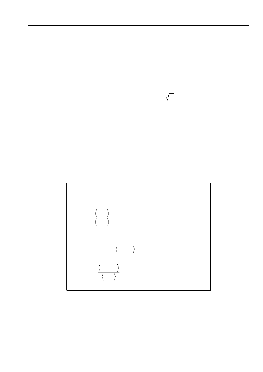
Code_Aster

Version

6.4

Titrate:

Linear Solvor of combined gradient type

Date

17/02/04

Author (S):

O. BOITEAU, J.P. GREGOIRE, J. PELLET

Key

R6.01.02-B

Page

29/44

Manual of Reference

R6.01 booklet: Iterative methods

HI-23/03/001/A

In the absolute, one can préconditionner a linear system by the left (“left preconditioning”), by
straight line (resp. “right”) or by making a mixture of both (resp. “Split”). It is this last version which goes
to be retained for our operator SPD, because one cannot directly apply the GC to solve

()

: even if

- 1

and

are SPD, it is not inevitably the case of their product.

The easy way then consists in using a matrix of prepacking SPD,

, for which one thus goes

to be able to define another matrix (

being symmetrical real, it is diagonalisable in the form

UDU

with

()

diag

and

orthogonal matrix. Required matrix SPD

comes then from the associated decomposition

()

Udiag

)

1/2

such as (

1/2

)

. From where

the new problem of work, this time SPD

()

4 3

4 2

éq

4.1-2

on which one will be able to apply the standard algorithm of the GC to constitute one what is called
Gradient Combines Packaged (GCPC).

Algorithm

In short, in substituent in the algorithm 4, expressions of the preceding problem

()

and while working

a little with simplification the whole to handle only expressions in

and

, it occurs it

following unfolding.

dd)

(news

)

optimal

conjugaiso

parameter

(

onné)

préconditi

ésidu

(

)

example

(

via

stop

Test

)

residue

new

(

)

reiterated

new

(

)

descent

optimal

parameter

(

Loop

given,

tion

Initialized

)

(

)

(

)

(

)

(

)

(

)

(

)

(

)

(

Algorithm 5: Packaged combined gradient (GCPC).

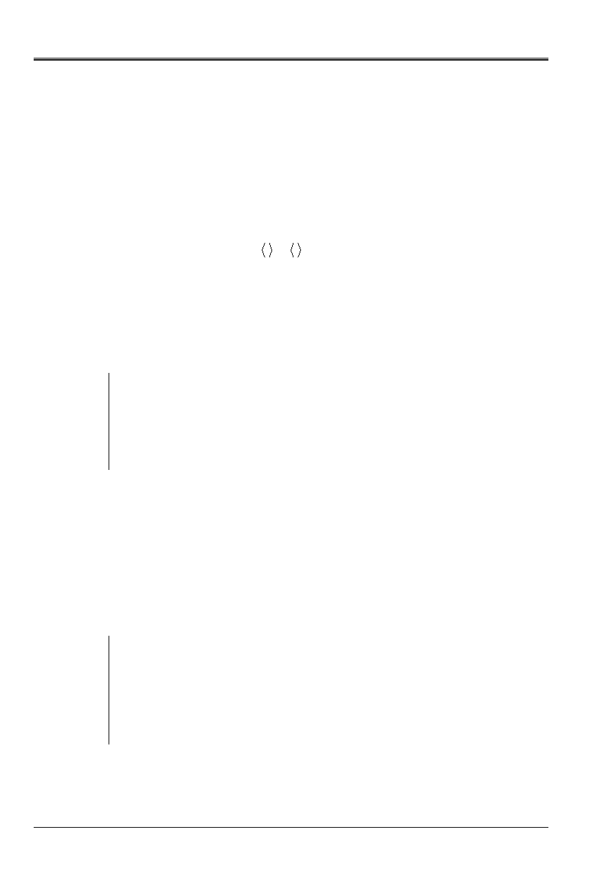
Code_Aster

Version

6.4

Titrate:

Linear Solvor of combined gradient type

Date

17/02/04

Author (S):

O. BOITEAU, J.P. GREGOIRE, J. PELLET

Key

R6.01.02-B

Page

30/44

Manual of Reference

R6.01 booklet: Iterative methods

HI-23/03/001/A

But makes some, the symmetrical character of the initial packaged problem

()

is quite relative. It is

indissociable of the subjacent scalar product. If instead of taking the usual Euclidean scalar product,
one uses a definite matric scalar product compared to

- 1

, it is possible to symmetrize it

packaged problem which was not it initially. As for the methods of Krylov into modal,
it is the couple (operator of work, scalar product) which it is necessary to modulate to adapt to the problem!
Thus,

- 1

being symmetrical compared to

- scalar product, one can substitute this new

operator of work and this new scalar product in the algorithm of the nonpackaged GC
(algorithm 4)

And (O surprised!) by working the expressions a little, one finds the algorithm of the GCPC exactly
precedent (algorithm 5). One proceeds in the same way with a prepacking on the right,

- 1

, via one

- 1

- scalar product. Therefore, prepacking on the right, on the left or “splitté with mode SPD”,

all lead rigorously to the same algorithm. This observation will be useful for us thereafter
when one realizes that the matrices provided by Code_Aster (and as the préconditionneurs as one
their will associate) are not always in conformity with the ideal scenario

()

Note:

· This alternative of the GCPC, which by far is spread, is sometimes called in

literature

: packaged combined gradient not transformed (`untransformed

preconditioned conjugate gradient'). In opposition to the transformed version which handles
clean entities of the new formulation.

· General methods of descent and, particularly nonlinear GC,

also préconditionnent (cf [§2.3]). This time with an approximating preconditionnor
the reverse of Hessien at the point considered, so as to make spherical the graph of
functional calculus in the vicinity of this point.

Overflight of the main préconditionneurs

The solution often adopted for its simplicity of implementation, his report/ratio “effectiveness
numerical/overcost calculation “for problems too badly not conditioned, consists with préconditionner
by the diagonal of the initial operator

()

diag

éq

4.1-3

It is what is called the diagonal prepacking or of Jacobi (JCG for `Jacobi Conjugate
Gradient') by reference to the iterative method of resolution of system linear of the same name.

Note:

· It is the solution often adopted in mechanics of the fluids [Gre97] (N3S, Code_Saturne),

where the process of Uzawa naturally produces a well conditioned problem, and which made
fame of the JCG, transformed for the occasion into true “animal of race” dedicated to
large computers: vectorization, parallelization, management of the covers and the memories…

· It is a solution suggested, in mechanics of the structures, by good numbers of codes

commercial: ANSYS, Zébulon, Nastran (cf [bib4] [§8.3]). It was presents in
Code_Aster but its unreliability led to its resorption.

· This principle of preconditionnor “of poor” extends to the methods of descent in

taking this time the diagonal of Hessien.

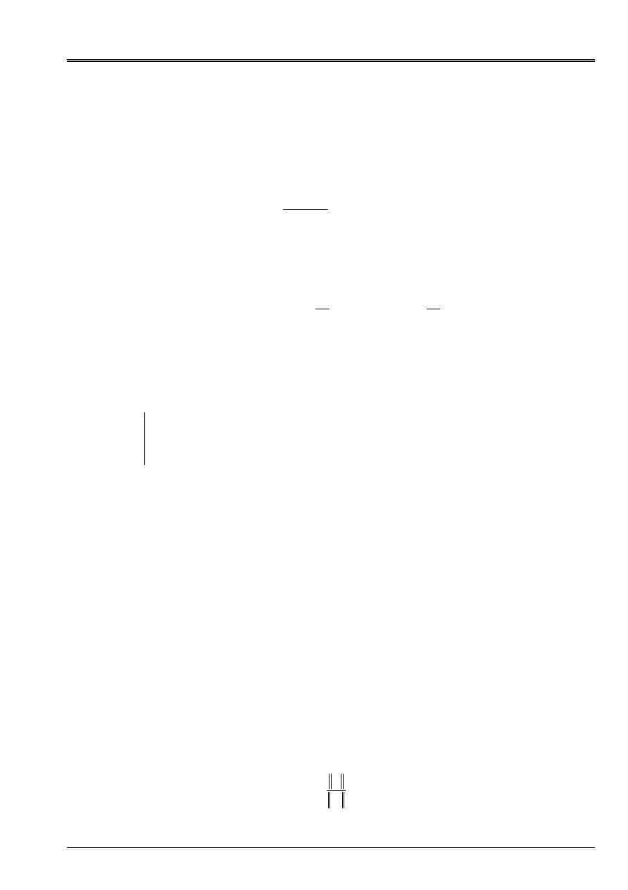
Code_Aster

Version

6.4

Titrate:

Linear Solvor of combined gradient type

Date

17/02/04

Author (S):

O. BOITEAU, J.P. GREGOIRE, J. PELLET

Key

R6.01.02-B

Page

31/44

Manual of Reference

R6.01 booklet: Iterative methods

HI-23/03/001/A

Another very widespread preconditionnor is the SSOR (for Symetric Succesive Over Relaxation).
Like the precedent, it is deduced from an iterative method “ancestral”: method of Gauss-Seidel
released. By breaking up the initial operator in the usual form

where

is its

diagonal and

its strictly lower triangular part, it is written (according to the parameter

relieving

)

()

(

) (

)

(

)

SSOR

éq

4.1-4

It has the advantage of not requiring report storage and of overcost calculation, since it is
directly elaborate from

, while being very simple to reverse (an descent-increase). On

model problems (famous “the Laplacian on the square unit”) of the theoretical results were
exhumed in finite elements

()

(

)

éq

4.1-5

In addition, it with faculty, for an operator SPD, to fix quotas for his spectrum in the tape

]]

However, it proved in practice industrial, less effective than the préconditionneurs of
incomplete Cholesky type which we will approach in the following paragraph. And it poses the problem
delicate of the choice of the parameter of optimal relaxation, by nature very “problem-dependant”.

Note:

· This preconditionnor was proposed by D.J.Evans (1967) and was studied by O.Axelsson (1974).

He declines himself in grinds versions: nonsymmetrical, by blocks, with parameter of relieving
optimal…

· While posing

=1 one finds the particular case of Symmetrical Gauss-Seidel

()

(

)

(

)

SGS

- 1

éq

4.1-6

A string of other préconditionneurs thus was born since about thirty years in
literature: especially polynomial [bib7], [bib34] but also ACP, ADI, ADDKR, by elements…. Some
are specific of an application, others more general. The “effects of modes” also made them
work! For more information one will be able to consult the monumental sum made by G.Meurant
[bib27] or books of Y. Saad [bib35] and H.A. Van der Vorst [bib40].

4.2

Incomplete factorization of Cholesky

Principle

One has just seen that the préconditionneurs is often inspired by linear solveurs with whole share:
Jacobi for that diagonal, Gauss-Seidel for SSOR. That based on an Incomplete factorization of
Cholesky (IC) does not escape the rule! But it is based this time, not on another method
iterative, but on his/her “enemy brother”, a direct method of Cholesky type. From where denomination
ICCG (“Incomplete Cholesky Conjugate Gradient”) given to the coupling of this preconditionnor
with the GCPC.

The initial operator being SPD, it admits a decomposition of Cholesky of the type

where

a lower triangular matrix. One calls incomplete factorization of Cholesky, the search for one
stamp

triangular lower as digs as possible and such as

that is to say near to

in one

feel to define. For example, while posing

one will ask that the relative error (expressed

in a matric standard with the choice)

éq

4.2-1

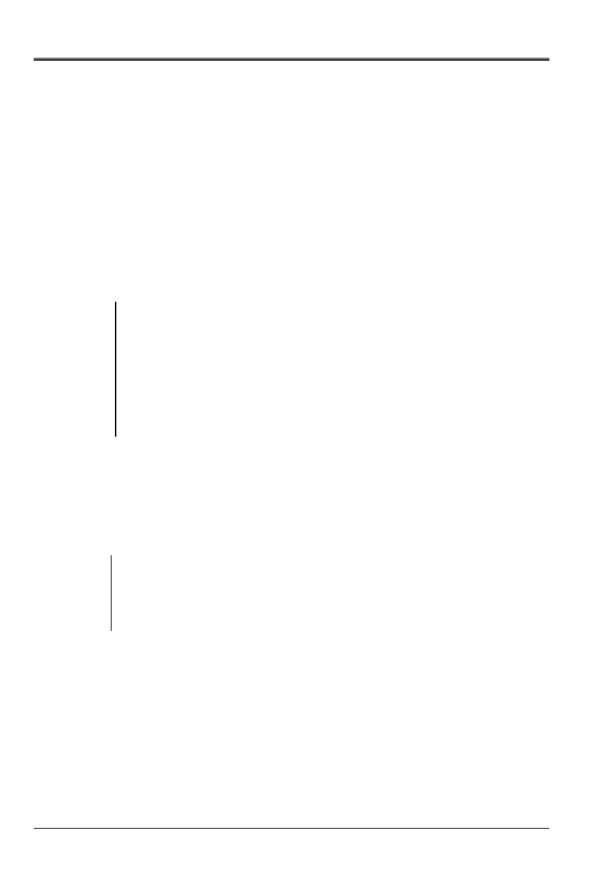
Code_Aster

Version

6.4

Titrate:

Linear Solvor of combined gradient type

Date

17/02/04

Author (S):

O. BOITEAU, J.P. GREGOIRE, J. PELLET

Key

R6.01.02-B

Page

32/44

Manual of Reference

R6.01 booklet: Iterative methods

HI-23/03/001/A

that is to say smallest possible. With the reading of this “rather evasive” definition one foresees the profusion of
possible scenarios. Each one went there from its own incomplete factorization! The work of G.Meurant
[bib27] great diversity shows some: IC

(

, MIC

(

, released, reordered, by blocks….

However, to be simplified the task, one forces often a priori the structure digs

, i.e.

its graph

() ()

{

}

éq

4.2-2

It is obviously a question of finding a compromise: the more this graph will be extended and the more the error [éq 4.2-1]
will be small but more calculation and storage of what is not (in the case which interests us) only one
preconditionnor will be expensive. Generally, the préconditionneurs are recursive and in their
basic level, they impose on

the same structure as that of

() ()

Note:

· Initially, these incomplete factorizations were developed to solve

repeatedly a linear system of type

)

Drunk

éq

4.2-3

The “nerve of the war” being then the spectral radius

()

[

]

that a judicious choice

()

can notably contribute to make fall.

· This principle of incomplete factorization spreads without sorrow with the standard case where

the operator is written

with this time

. One speaks then about factorization

Incomplete of type LU (ILU

for “Incomplete LU”).

Strategy retained in Code_Aster

It is about a preconditionnor of the type

ILU

(because we will see in the paragraph according to whether the matrices

of work of Code_Aster often lose their definite-positivity) inspired of work of H. Van DER
Vorst [bib40]. The matrices remaining however symmetrical, one can write

LDL

and

LDL

Note:

The matrix not being regular simply symmetrical SPD but one is not, a priori,
ensured of the existence of one factorized

LDL

without having recourse to permutations of lines

and of columns (

Km No

LDL

with

stamp permutation). Scenario which was not envisaged in

no linear solveurs of Code_Aster and that, in any event, MORSE storage of
matrices of the prohibited GCPC. Fortunately, it will be seen that a happy combination of circumstance
allows to resolve the situation (cf [§5.1])!

In any rigor one should speak about incomplete factorization of type ILDLT but in the literature and
in documentations of the codes, one amalgamates already ILU and IC, even their alternatives, it are not thus
not the sorrow to enrich the list by the acronyms

This incomplete factorization, in the line line of the preceding theoretical recalls, rests on
two official reports which we now will support:

· concept of filling by levels,

· low magnitude of the terms resulting from this filling.

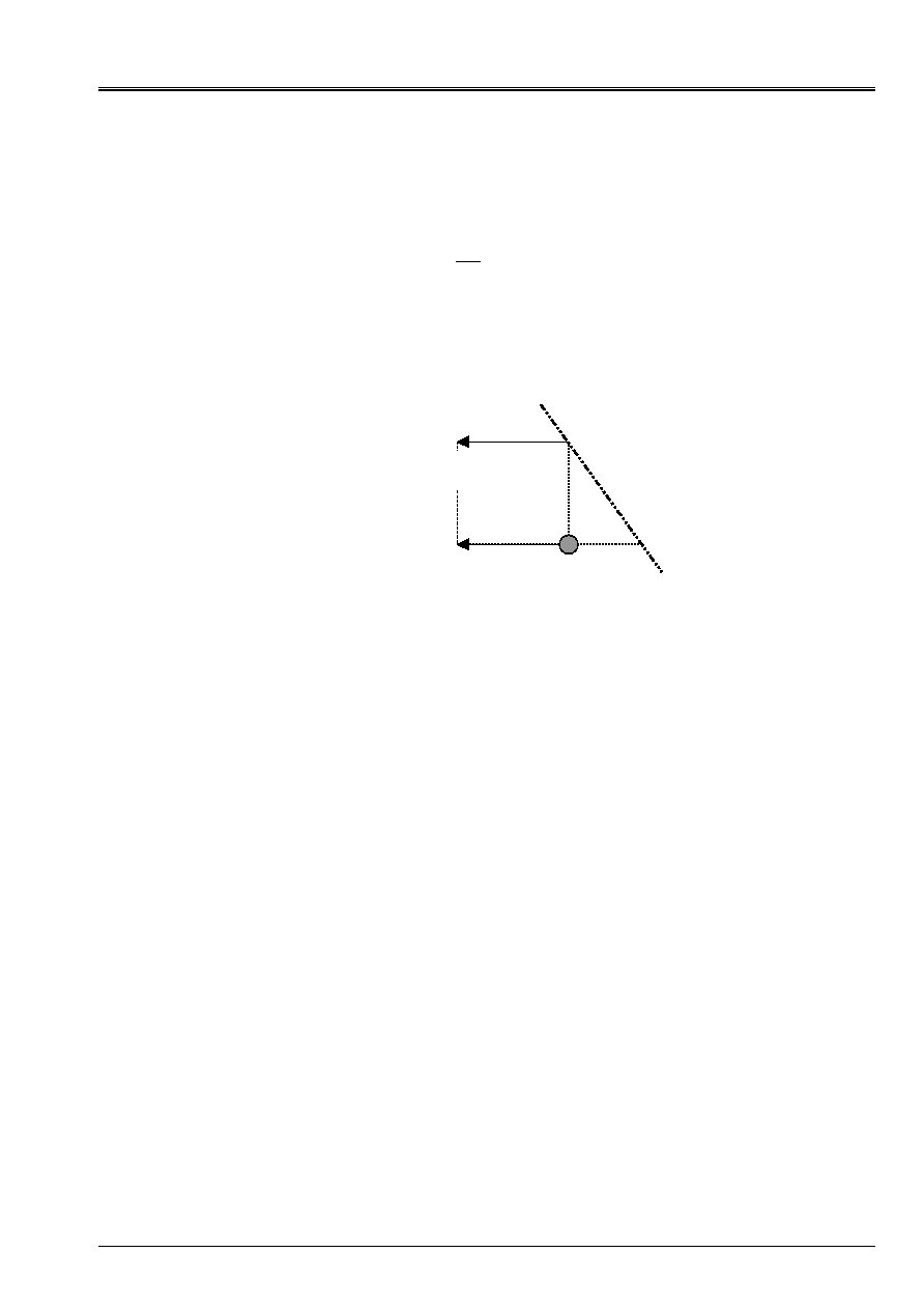
Code_Aster

Version

6.4

Titrate:

Linear Solvor of combined gradient type

Date

17/02/04

Author (S):

O. BOITEAU, J.P. GREGOIRE, J. PELLET

Key

R6.01.02-B

Page

33/44

Manual of Reference

R6.01 booklet: Iterative methods

HI-23/03/001/A

Filling by levels

The construction of factorized is carried out, line by line, via the usual formula

éq

4.2-4

From where the phenomenon of progressive filling of the profile (“English rope”): initially the matrix

with

the same filling as stamps it

, but during the process, the null term of

can

to correspond a term not no one of

. It is enough that there is a column

) comprising a term not

no one for the lines

and

(cf [Figure 4.2-a]).

Appear 4.2-a: Phenomenon of filling during factorization.

Besides these nonnull terms being able them same to correspond to former fillings, from where
a concept of level of recursivity which can be interpreted like as many “levels” of filling.
One will speak thus about factorized incomplete of level

(stored in

L (0)

) if it reproduces with

identical the structure (but of course not values which is different) diagonal part
lower strict of

(i.e the same graph). Factorized level 1 (resp.

L (1)

) will be able it to include

filling led by nonnull terms of

(noted terms

in [Figure 4.2-b]), that of

level

(resp.

L (2)

) will be able to mingle the new nonnull terms with it (

) preceding to constitute

possible new terms (noted

), and so on recursively…

This is illustrated on the academic case of a matrix digs pentadiagonale resulting from the discretization
differences finished of the Laplacian on a uniform grid 2D (cf [Figure 4.2-b]). One only represents any
structure:

, diagonal terms spectators,

, terms initially nonnull,

, terms filled with

the stage n°

The factorized incomplete one

L (3)

conduit here with a complete filling, the relative error will be then null

and the GCPC converges in an iteration. The interest of the exercise is of course purely didactic!

New

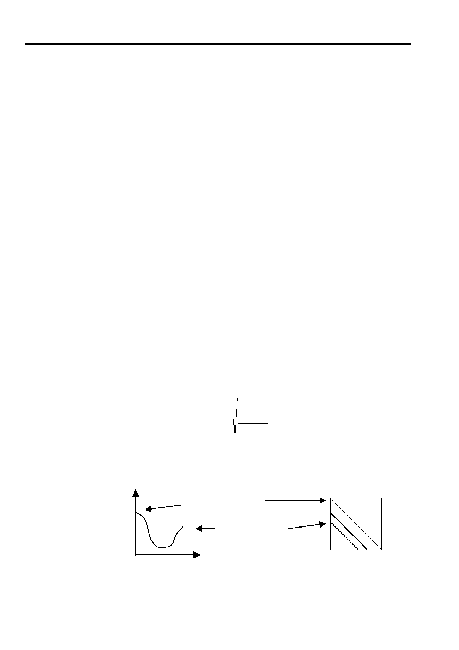
Code_Aster

Version

6.4

Titrate:

Linear Solvor of combined gradient type

Date

17/02/04

Author (S):

O. BOITEAU, J.P. GREGOIRE, J. PELLET

Key

R6.01.02-B

Page

34/44

Manual of Reference

R6.01 booklet: Iterative methods

HI-23/03/001/A

()

sym

Appear 4.2-b: Structure of the various factorized incomplete ILU

(p)

on the academic case of the Laplacian.

Low magnitude of the terms resulting from the filling

In addition, one empirically notices a very interesting property of these new terms
resulting from the filling: their absolute value decrease while moving away from the areas already filled by
nonnull terms of

. Maybe, in the preceding case, of the main under-diagonal and that external.

To be convinced some it is enough to visualize the following function (cf [Figure 4.2-c])

()

log

éq

4.2-5

who represents the orders of magnitude of the terms of

ième

under-diagonals. For example

y (0)

corresponds to the main diagonal.

Appear 4.2-c: Relative importance of the diagonals of

External diagonal

y (K)

Main diagonal

k+i, I

Number of the under-diagonal

Function amplitude
terms
under-diagonal

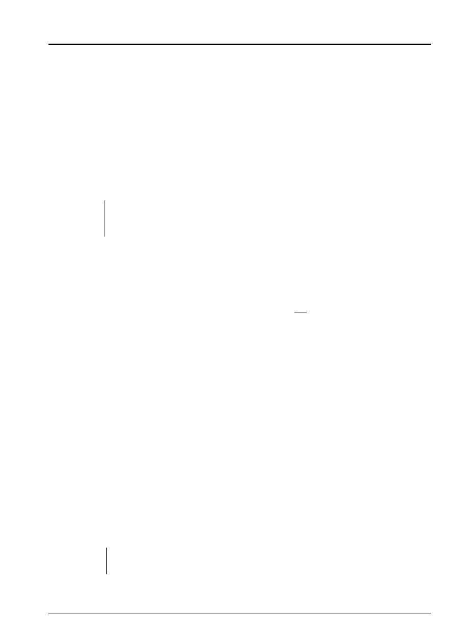
Code_Aster

Version

6.4

Titrate:

Linear Solvor of combined gradient type

Date

17/02/04

Author (S):

O. BOITEAU, J.P. GREGOIRE, J. PELLET

Key

R6.01.02-B

Page

35/44

Manual of Reference

R6.01 booklet: Iterative methods

HI-23/03/001/A

If one recapitulates, one thus has:

· level of a recursive and skeletal filling,

· a less importance of the terms corresponding to high levels of filling.

From where a certain “full power” left with incomplete factorizations ILU

(

neglecting these terms

medians. This approximation “cheaply” of

- 1

will be used then as preconditionnor in

algorithm 5 of the GCPC (

- 1

). To preserve a certain interest at the thing (if not as much

to solve the problem directly!), one limits oneself to the first levels of filling:

=0, 1, 2

even 3. All depends on the number of linear systems which one will have to solve with the same matrix.

Note:

· There exists little of theoretical results on this type of preconditionnor. What does not prevent it

not to appear often effective [bib22].

· It is a solution suggested, in mechanics of the structures, by considerable large

codes: ANSYS, Zébulon, Nastran, Code_Aster (cf [bib4] [§8.3]).

Complexity and occupation memory

As regards the cost additional calculation with one factorized incomplete, it is very difficult at
to estimate and, in practice, depends largely on the way in which it was coded (with our
knowledge, there do not exist theoretical results on the thing). With a low level of

filling, one hopes only that it is much lower than

of a complete factorization.

Because a compromise is to be found between occupation memory and complexity. To constitute these
factorized incomplete, it is often necessary to allocate temporary workspaces. Thus, in
establishment of prepacking ILU

(

of Code_Aster, it was selected to facilitate the algorithmic one

(sorting, search of indices and coefficients in the profile, management of the recursivity and the filling…)
by creating matrices temporarily representing storage full with the initial matrix and sound
filling.
With this temporary workspace, additional storage due is added of course to
final preconditionnor. On the level

, it is theoretically at least of the same command as that of

stamp. From where minimal effective a memory complexity of the GCPC of

(

)

realities and

(

)

Cn 2

entireties. When one goes up in complétude, only the practice can bring a pretense

of answer.

In short, one empirically shows with Code_Aster, that an overall dimension memory should be envisaged
total of

(

)

realities and

(

)

Cn 2

entireties with

=2,5 in ILU

(0)

(level by defect in Code_Aster),

=4,5 in ILU

(1)

=8,5 in ILU

(2)

For more precise details on the data-processing establishment of the GCPC in Code_Aster and its use on
case-tests quasi-industrialists, one will be able to consult the notes [bib22] or [bib3].

Note:

In Code_Aster, the overall dimension memory of an entirety is identical to that of a reality and, for
the GCPC, no reservation of place or pagination memory could installation.
What does not arrange anything!

Code_Aster

Version

6.4

Titrate:

Linear Solvor of combined gradient type

Date

17/02/04

Author (S):

O. BOITEAU, J.P. GREGOIRE, J. PELLET

Key

R6.01.02-B

Page

36/44

Manual of Reference

R6.01 booklet: Iterative methods

HI-23/03/001/A

5 Establishment

Code_Aster

5.1 Difficulties

particular

Taking into account of the limiting conditions

In Code_Aster, there are two manners of taking into account the boundary conditions and this stage
be carried out during the effective construction of the matrix of rigidity:

· By double dualisation [bib30] (operators AFFE_CHAR_ACOU/MECA/THER) while using

ddls specific, known as of Lagrange, which includes the groups of unknown factors concerned and
allow to check all types of linear limiting conditions (Dirichlet generalized)

You

éq 5.1-1

with

real matrix of size

p X N

. This technique packs the matrix of rigidity in one

new matrix, known as “dualized”, which becomes the new matrix of work

)

éq

5.1-2

where

and

are two strictly positive realities.

· By simple elimination of the unknown factors (operators AFFE_CHAR_CINE) in substituent and in

carrying out the setting zero have of

lines and columns concerned of the matrix of rigidity. This

is valid only for blockings of ddls, one cannot thus take into account
linear relation. The matrix of rigidity is written then

)

éq

5.1-3

while noting

its unchanged part.

Each of the two approaches has its advantages and its disadvantages: generics, modularity but
increase in the size of the problem, degradation of its conditioning and loss of its definite
positivity for the first. Contrary to the second which decreases by it the size but which is circumscribed
with certain types of limiting conditions and is, by means of computer, more delicate to implement.
In Code_Aster, primacy being given to the facility of use like to the contingencies
numérico-data processing of robustness, establishment, of maintenance and evolutionarity, it is clearly
the first approach which was privileged.

Note:

Other approaches were possible: simple dualisation, taken into account of
conditions limit in the variational formulation, combined gradient projected (GCP cf [bib4]
[§6.2.3])…

Code_Aster

Version

6.4

Titrate:

Linear Solvor of combined gradient type

Date

17/02/04

Author (S):

O. BOITEAU, J.P. GREGOIRE, J. PELLET

Key

R6.01.02-B

Page

37/44

Manual of Reference

R6.01 booklet: Iterative methods

HI-23/03/001/A

Consequence on the GCPC

With AFFE_CHAR_CINE, the operator of work

remaining SPD, all the theory recalled in

preceding paragraphs applies. On the other hand, with AFFE_CHAR_ACOU/MECA/THER (case more

frequent in practice), it is not any more the case, because it becomes simply symmetrical and loses its character
defined positive. The consequences are then of three types:

· The total convergence of the GCPC (cf [éq 3.2-9]) is not guaranteed any more,

· When it occurs, it is slowed down (cf [éq 3.2-11]) by a degraded conditioning

()

)

· Prepacking cannot be carried out any more via one IC

(

, but rather by a ILU

(

(cf [§4.2]). It is necessary still that factorization

LDL

that is to say always possible without having with

to permute line or column!

Fortunately, an adequate provision of the multipliers of Lagrange compared to the groups of
ddls that they concern (they must include these ddls cf [bib30] [§4]), allows to obtain without blow to férir
this incomplete factorization. B.Nitrosso [bib29] thus showed that it is stable and that, in addition,
used as a preconditionnor, it restores the total convergence of the GCPC (ouf!).

Note:

· In this same report/ratio, B.Nitrosso shows that diagonal prepacking is not

possible (cf [§4.1]), because it leads to the cancellation of the scalar product to the denominator
stage (7) of algorithm 5: calculation of the optimal parameter of conjugation. Therefore,
contrary to N3S and Code_Saturne, Code_Aster cannot propose this option
not very reliable.

· It does not remain about it less, that with dualized limiting conditions, the conditioning of

the operator of work is degraded and thus, the convergence of the slowed down GCPC. Others
commercial codes, with the instart of ANSYS [bib31], already made this official report.

Overall dimension memory

Taking into account the elements of [§4.2] and owing to the fact that in Code_Aster, an entirety has the same one
overall dimension memory that a reality (8 bytes), effective memory complexity of the GCPC is of at least

size of

with

=2,5 in ILU

(0)

(level by defect in Code_Aster),

=4,5 in ILU

(1)

=8,5 in ILU

(2)

In addition, contrary to the direct solveurs, the GCPC could not profit from a pagination because, on
this point, the its algorithmic dessert: all the matric blocks are used a great number of times,
in fact with each iteration, via the product matrix-vector.
Moreover, contrary has what was made in N3S, with the definition of the calculation case (mesh,
materials, loadings and conditions limit…), one does not hold, by advance, part of
memory to store there the vectors required by the GCPC. Therefore, progressively with the execution of
operators of the command file, the memory becomes a “true Gruyere” where it becomes difficult
to insert large objects.
The pagination of the direct solveurs enables them to cross without too many difficulties this shelf… it is
of course differently of the GCPC. From where, according to the sequence of the controls, an inflation of the sizes
necessary memories to make function its “job” with METHODE=' GCPC'. It is thus advised of
to work in mode “CONTINUATION” and to fix quotas for the resolution of the linear system at the head files

of control: the memory to the maximum will be thus preserved.
If the going beyond report is modest, one can also try to fix quotas for this phenomenon
of crumbling by modifying the parameter setting of management memory via the parameter setting (key words factor
MEMORY, key words MANAGEMENT, TYPE_ALLOCATION or PARTITION) of the control BEGINNING

[U4.11.01].

Code_Aster

Version

6.4

Titrate:

Linear Solvor of combined gradient type

Date

17/02/04

Author (S):

O. BOITEAU, J.P. GREGOIRE, J. PELLET

Key

R6.01.02-B

Page

38/44

Manual of Reference

R6.01 booklet: Iterative methods

HI-23/03/001/A

Let us notice all the same that storage MORSE (It is also voted by plebiscite by the multifrontale.
solvor of Gauss uses, as for him, a “rough” storage more, SKYLINE (“line of sky” in good

French!), which allows an easier management of the filling but amplifies the occupation memory)
matrices and of the vectors chosen for the GCPC makes it possible to manage the hollow character as well as possible of
operators and thus, limit the overall dimension memory.

Parallelization

Contrary to the multifrontale, the GCPC was not paralleled. This work was however already carried out
[bib20], [bib23], but only for one diagonal prepacking (cf [§4.1-3]) because it poses
problems of effective parallel construction of the preconditionnor in order not to disturb the others
stages.
With these problems of “parallel preconditioning” are added strong data-processing contingencies in
disrtribuées memories. For more information and references on this parallelism known as
“numerical” and his réminicences in Code_Aster, one will be able to consult [bib4] [§3].

5.2 Perimeter

of use

List Code_Aster controls which can use GCPC:

· CALC_FORC_AJOU,
· CALC_MATR_AJOU,

· CALC_PRECONT,
· Possible DYNA_NON_LINE symmetrized Approximation (cf [§5.3]),

· DYNA_TRAN_EXPLI possible symmetrized Approximation,
· Possible MACR_ASCOUF_CALC symmetrized Approximation,
· MACR_ASPIC_CALC possible symmetrized Approximation,

· MACRO_MATR_AJOU,
· MACRO_MATR_ASSE,

· MECA_STATIQUE,
· NUME_DDL,
· Possible STAT_NON_LINE symmetrized Approximation,

· THER_LINEAIRE,
· THER_NON_LINE possible symmetrized Approximation,
· Possible THER_NON_LINE_MO symmetrized Approximation.

5.3

Symmetrical character of the operator of work

If the matrix is not symmetrical two cases of figures present. That is to say the linear solvor is inserted
in a non-linear process (operators mentioned cf lists [§5.2]), that is to say the aforementioned is linear (them
other operators).
In the first case, one transforms the initial problem

in a new symmetrized problem

(

)

. One supposes by there that the nonlinear solvor including (algorithm of Newton) goes

to compensate for the approximation of the initial operator by

(

)

= 21

. It is not besides only

approximation of this nonlinear process… the choice of the tangent matrix in is, for example, one
other. This symmetrized approximation does not harm the robustness and the coherence of the unit and
avoid a more expensive nonsymmetrical resolution. This operation is carried out by activating the word
key SYME = “YES” (by defect “NOT”) of the key word factor SOLVEUR and it is licit for the three
linear solveurs of the code: “LDLT”, “MULT_FRONT” and “GCPC”.

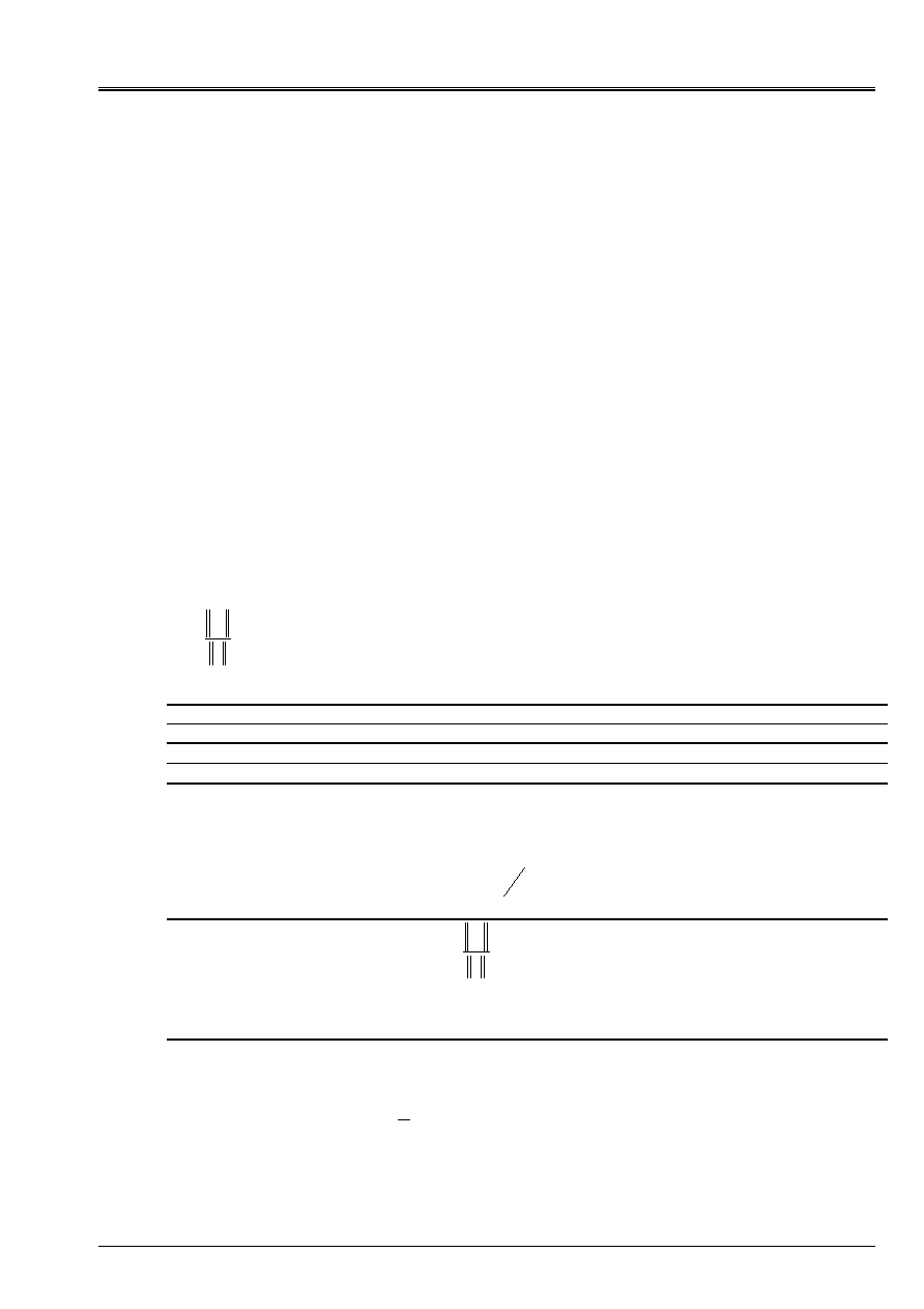
Code_Aster

Version

6.4

Titrate:

Linear Solvor of combined gradient type

Date

17/02/04

Author (S):

O. BOITEAU, J.P. GREGOIRE, J. PELLET

Key

R6.01.02-B

Page

39/44

Manual of Reference

R6.01 booklet: Iterative methods

HI-23/03/001/A

When the problem is purely linear, one can await no compensation of one
unspecified including process and this approximation become impossible. Resorts to the GCPC
currently in Code_Aster (it is illicit would be necessary to call upon some of its alternatives: GMRES,
Orthomin, double GC, normal equation…) and it is necessary to reverse this nonsymmetrical system via LDLT' or
“MULT_FRONT”. The nature of the operator of work is detected automatically, no one is not need for
to notify via key word SYME.

5.4

Parameter setting and display

To activate this functionality, it is necessary to initialize the key word METHOD with “GCPC” in the key word factor
SOLVEUR [U4.50.01].

Only the prepacking of incomplete the Cholesky type is available and it is not possible of
to exempt: NIVE_REMPLISSAGE=0 thus does not mean “

without prepacking

” but

prepacking of the type ILU

(0)

To minimize the size of the profile of the matrix of work and its preconditionnor, an algorithm of
renumerotation is available by defect: “RCMK” for “Reverse Cuthill Mac-Kee” (cf [bib26] [§5.4.2]).
It is nevertheless désactivable.
In “exploiting” the level of complétude of prepacking, one can modify the compromise
“time calculation/occupation memory”.
Contrary to the direct methods, it was necessary to fix a maximum iteration count discriminating them
iterative calculations converged of not converged. This threshold (skeletal) is arbitrarily fixed at
half of the ddls of the problem of work

)

. If at the end of

=NMAX_ITER stages, the relative residue

is not lower than RESI_RELA, calculation stops in ERREUR_FATALE.

Key word factor

Key word

Default value

References

SOLVEUR METHODE=' GCPC'

“MULT_FRONT”

[§1]

PRE_COND=' LDLT_INC' “LDLT_INC”

[§4.2]

NIVE_REMPLISSAGE=0,1,2… 0 [§4.2]

RENUM=' RCMK' or “WITHOUT” “RCMK”

NMAX_ITER=

max

, a number

iterations maximum
acceptable.
If

max

=0, fixed

automatically with

[Algorithm 5]

RESI_RELA=

, value

maximum of the residue relative to
convergence (with

ème

iteration).

- 6

[Algorithm 5 and
[§3.3]

SYME=' OUI' or “NOT”

Approximation symmetrized of
the operator of work by

(

)

= 21

Sell by auction only in not
linear

“NOT”

[§5.2/3]

Table 5.4-1: Summary of the parameter setting of the GCPC.

Code_Aster

Version

6.4

Titrate:

Linear Solvor of combined gradient type

Date

17/02/04

Author (S):

O. BOITEAU, J.P. GREGOIRE, J. PELLET

Key

R6.01.02-B

Page

40/44

Manual of Reference

R6.01 booklet: Iterative methods

HI-23/03/001/A

To be complete on the parameter setting and the display in the file message (.mess), let us mention:

· Value INFO=2 traces the evolution of the standards of the residues absolute

and relative

, thus

that the correpondant number of iteration,

, as soon as it decrease from at least 10% (not

skeletal).

· Value INFO=3 traces these evolutions with each iteration.

· With convergence, i.e. as soon as

RESI_RELA

, one recalls in more the value of

normalizes initial absolute residue

5.5 The Councils

of use

Like one recalled it already many times, in Code_Aster a whole series of factors calls into question
the main “historical” advantages concurentiels (cf [§1]) of the GCPC compared to its alter-egos
direct:

· Efforts made to paginate as well as possible the resources memories required by the solveurs

direct (pagination supplements for “LDLT” and partial for “MULT_FRONT”).

· Not required of a strategy of swivelling which allows a hollow storage of the matrix of

work (MORSE for “MULT_FRONT” and SKYLINE for “LDLT”).

· An optimized management of the filling for “MULT_FRONT” (full frontal matrices).
· Parallelization in memory shared for “MULT_FRONT” (cf [bib33] or [bib4] [§3.2]).

· The matrix of work is assembled beforehand and stored before resorts to the solvor.

· Bad conditioning generally noted in mechanics of the structures worsened by

taking into account of Dirichlet generalized via of Lagranges (cf [§5.1]).

All in all, the best compromise robustness/overall dimension memory/cost CPU seems to return
[bib3] with the method by defect of key word SOLVEUR: the multifrontale. However, for problems

conditioned rather well (thermal [bib1], simple geometry with a mesh and characteristics
materials relatively homogeneous…) or very greedy in memory (several million ddls), it
GCPC can prove to be an interesting alternative.

Because of its natural modularity and simplicity of its components (produced matrix-vector and
scalar product), it remains nevertheless much simpler to maintain and make evolve/move that the others
direct solveurs. It is the solvor “passes everywhere” easy to establish (at least in its version of
base) and very teaching. He is often connected in more general processes (solveurs
encased, solveurs of interface of the decomposition of fields…) or adapted, on a case-by-case basis, for
structures of particular matrices.

In addition, a property not exploited yet in the official version of Code_Aster, its scalability
intrinsic, a parallelization accredits on a great number of processors. Whereas for
same numbers of processors, the speed-ups of the direct methods worsen largely.
It is one of the reasons which led to often retaining the GCPC as solvor of interface for
methods of decomposition of fields [bib4].

The small last favors GCPC, which had historically its importance, can lie in the fact
that it accumulates less the round-off errors than its direct competitors. They are circumscribed with
last iteration whereas the direct methods accumulate them during factorization. This known as
they indirectly are found when convergence is long in coming and that the generated residues are not
more completely orthogonal!

Code_Aster

Version

6.4

Titrate:

Linear Solvor of combined gradient type

Date

17/02/04

Author (S):

O. BOITEAU, J.P. GREGOIRE, J. PELLET

Key

R6.01.02-B

Page

41/44

Manual of Reference

R6.01 booklet: Iterative methods

HI-23/03/001/A

In short, the GCPC established in Code_Aster offers a compromise robustness/complexity
calculation/memory less powerful than the multifrontale. Nevertheless, this general official report is undoubtedly with
to balance, as well it is true as it renders enormous services in other fields of physics: N3S,
TRIFOU, Code_Saturne, LADYBIRD, ESTET….
One can try to synthesize, from a point of view “user of Code_Aster” the inventory of fixtures
precedent, in the table below.

Solveurs

Cut problem

Robustness Memory

CPU

Parameter setting

Maintainability

Small
case
(<10

DDL)

Case
standards
(<10

DDL)

Very
large
case
(>10

DDL)

MULT_FRONT
DEFECT

Excellent

Because of
pagination:
weak

Good

Nothing to make

Standard

not

yes

To see

LDLT

Excellent

Because of
pagination:
also weak
that one wants

Expensive Nothing to make

Enough easy

yes

not

prohibited

GCPC

Very variable Very variable Very

variable

To adapt to
individually

Easy yes

With

to see

Yes in
thermics

Yes?

Table 5.5-1: Summary of the linear solveurs in Code_Aster.

Code_Aster

Version

6.4

Titrate:

Linear Solvor of combined gradient type

Date

17/02/04

Author (S):

O. BOITEAU, J.P. GREGOIRE, J. PELLET

Key

R6.01.02-B

Page

42/44

Manual of Reference

R6.01 booklet: Iterative methods

HI-23/03/001/A

6 Bibliography

[1]

NR. ANFAOUI: A study of the performances of Code_Aster: proposal for an optimization.
Training course of of mathematics applied of PARIS VI (2003).

[2]

O. BOITEAU: Algorithm of resolution for the generalized problem. Doc. of Code_Aster
available on the site (http://www.code-aster.org), [R5.01.01] (2000).

[3]

O. BOITEAU: Analyze establishment of the gradient combined in Code_Aster and tests
other alternatives via library CXML. CR-I23/03/014 (2003).

[4]

O. BOITEAU: Decomposition of field and parallelism in mechanics of the structures: State
art and benchmark for an establishment reasoned in Code_Aster. HI-23/03/009
(2003).

[5]

J.F. BONNANS, J.C. GILBERT, C. LEMARECHAL & C. SAGASTIZABAL: Optimization
numerical: theoretical and practical aspects. ED. Springer collection mathematics &
applications, 27 (1997).

[6]

A. BOURAS, V. FRAYSSE & L. GIRAUD: With relieving strategy for inner-outer linear solvers
in DD methods. Report/ratio CERFACS TR/AP/00/17 (2000).

[7]

T. BUFFARD & J.M. HERARD: A method of polynomial prepacking for
systems SPD. HE-41/89.16 (1989).

[8]

F. CHAITIN-CHATELIN & T. MESKAUSAS: Inner-outer iterations for solvers mode in
structural mechanics: application to Code_Aster. (2001).

[9]

F.CHAITIN-CHATELIN & T.MESKAUSAS. Inner-outer iterations for power method with
Chebyschev acceleration in neutronics. (2002).

[10]

B.A. CIPRA: The best off the 20th century: editors name top10 algorithms. SIAM News, 33-4
(2000).

[11]

J.C. CULIOLI: Introduction to optimization. ED. Ellipse (1994).

[12]

V. FRAYSSE: The power off backward error analysis. HDR of the National Institute
Polytechnic of Toulouse (200).

[13]

I. FRIED: Condition off finite element matrices generated from not uniform meshes. AIAA J.,
10 (1972), pp219-231.

[14]

G.H. GOLUB & V. LOAN: Matrix computations. ED. J.Hopkins University Close (1984).

[15]

G.H. GOLUB & D.P.O' LEARY: Summon history off the conjugate gradient and Lanczos
algorithms: 1948-1976. SIAM review, 31-1 (1989), pp50-102.

[16]

G.H. GOLUB & H.A. VAN DER VORST: Closer to the solution: Iterative linear solvers. The
state off the art in numerical analysis. ED. Clarendon close (1997), pp93-92.

[17]

G.H. GOLUB & Q. TESTSTEMYÈ: Inaccurate preconditioned conjugate gradient method with inner-outer
iteration. Report/ratio Stanford University, SCCM-97-04 (1997).

[18]

J.P. GREGOIRE: Algorithm of the GCPC for the resolution of a symmetrical linear system:
general presentation and instructions. HI/4333-07 (1982).

[19]

J.P. GREGOIRE: Effective vectorization of the GC in the case of hollow symmetrical matrices.
HI-72/6710 (1990).

[20]

J.P. GREGOIRE: Parallelization of the GC for matrices dig on CRAY C98.
HI-76/95/019 (1996).

Code_Aster

Version

6.4

Titrate:

Linear Solvor of combined gradient type

Date

17/02/04

Author (S):

O. BOITEAU, J.P. GREGOIRE, J. PELLET

Key

R6.01.02-B

Page

43/44

Manual of Reference

R6.01 booklet: Iterative methods

HI-23/03/001/A

[21]

J.P. GREGOIRE, C. ROSE & B. THOMAS: Direct and iterative solvers for finite-element
problems. Numerical algorithms, 16 (1997), pp39-53.

[22]

J.P. GREGOIRE: Acceleration of the convergence of the packaged gradient combined in
using incomplete factorization by level. HI-76/00/005 (2000).

[23]

J.P. GREGOIRE: Parallelization in memory distributed of the GC and the code user.
HI-76/01/007 (2001).

[24]

J.P. GREGOIRE: GCPC and fast calculation of the eigenvalues. HI-76/01/001 (2001).

[25]

P. JOLLY: Methods of combined gradient. N°84016 report/ratio of the lab. of numerical analysis of
PARIS VI (1984).

[26]

P. LASCAUX & R. THEODOR: Matric numerical analysis applied to the art of the engineer.
ED. Masson (1994).

[27]

G. MEURANT: Computer solution off broad linear systems. Studies in mathematics and its
applications, ED. Elsevier, 1999.

[28]

Mr. MINOUX: Mathematical programming, theory and algorithms. ED. Dunod (1983).

[29]

B. NITROSSO: Direct methods for hollow matrices SPD. Basic techniques with
the state of the art. HE-41/92.27 (1992).

[30]

J. PELLET: Dualisation of the boundary conditions. Doc. of Code_Aster [R3.03.01] (2001)
available on the site.

[31]

G. POOLE, Y.C.LIU & J. MANDEL: Advancing analysis capabilities in ANSYS though solver
technology. (2001) dispo. on site ANSYS.

[32]

C. ROSE: A parallel method multifrontale for the direct resolution of the systems
linear. HI-76/95/021 (1995).

[33]

C. ROSE: Method multifrontale. Doc. of Code_Aster [R6.02.02] (2001) dispo. on the site.

[34]

Y. SAAD: Practical uses off polynomial preconditionings for the conjugate gradient method.
Research report YALEU/DCS/RR-282, University of Yale (1983).

[35]

Y. SAAD: Iterative methods for sparse linear systems. ED. PWS, 1996.

[36]

Y. SAAD & H.A. VAN DER VORST: Iterative solution off linear system in the 20th-century.
J. comp. Appl. Maths., 123 (2000), pp35-65.

[37]

D. SELIGMANN: In connection with the methods of decomposition of the Gauss type. Doc. of
Code_Aster [R6.02.01] (1993) available on the site.

[38]

J.R. SHEWCHUK: Year introduction to the conjugate gradient method without the agonizing
bread. Report/ratio interns University of Carnegie Mellon (1994).

[39]

J.L. VAUDESCAL: Introduction to the methods of resolution of problems to the values
clean of large sizes. HI-72/00/01 (2000).

[40]

H. VAN DER VORST: Iterative broad Krylov methods for linear systems. ED. Cambridge
University Close (2001).