Velocity Potential

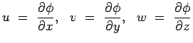
We have seen that for an irrotational flow $curl(\vec{V}) =0 or \nabla \times \vec{V}=0$ . It follows from vector algebra that there should be a potential such that

$\displaystyle \vec{V} = \nabla \phi$

(4.53)

$\phi$ is called the Velocity Potential. The velocity components are related to $\phi$ through the following relations.

$\displaystyle u = {{\partial \phi} \over {\partial x}}, v = {{\partial \phi} \over {\partial y}}, w = {{\partial \phi} \over {\partial z}}$

(4.54)

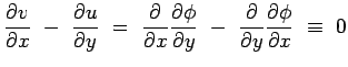
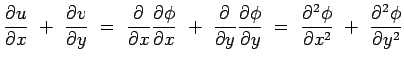
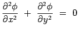
Velocity potential is a powerful tool in analysing irrotational flows. First of all it meets with the irrotationality condition readily. In fact, it follows from that condition. As a check we substitute the velocity potential in the irrotationality condition, thus,

$\displaystyle {\partial v\over {\partial x}} - {\partial u \over {\partial y}}... ... - {\partial \over {\partial y}}{ {\partial \phi} \over {\partial x}} \equiv 0$

(4.55)

The next question we ask is does the velocity potential satisfy the continuity equation? To find out we consider the continuity equation for incompressible flows and substitute the expressions for velocity coordinates in them. Accordingly,

$\displaystyle {\partial u\over {\partial x}} + {\partial v \over {\partial y}}... ...artial^2 \phi} \over {\partial x^2}} + {{\partial^2 \phi} \over {\partial y^2}}$

(4.56)

It is clear that to meet with the continuity requirements the velocity potential has to satisfy the equation,

$\displaystyle {{\partial^2 \phi} \over {\partial x^2}} + {{\partial^2 \phi} \over {\partial y^2}} = 0$

(4.57)

$\displaystyle \nabla^2 \phi = 0$

(4.58)

As with stream functions we can have lines along which potential $\phi$ is constant. These are called Equipotential Lines of the flow. Thus along a potential line $\phi = C$ .

The equation 4.58 is called the Laplace Equation and is encountered in many branches of physics and engineering. A flow governed by this equation is called a Potential Flow. Further the Laplace equation is linear and is easily solved by many available standard techniques, of course, subject to boundary conditions at the boundaries.

Note that in terms of velocity potential expression for circulation(Eqn. 4.45, see Circulation) assumes a simple form.

$\displaystyle \Gamma$	$\displaystyle = \oint_C \vec{V}\cdot d\vec{s}$
and
	$\displaystyle \vec{V} \cdot ds = \nabla \phi \cdot ds = d \phi$	(4.59)
giving
$\displaystyle \Gamma$	$\displaystyle = \oint_C d \phi$	(4.60)