|
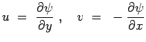
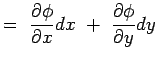
We notice that velocity potential  and stream function and stream function
 are connected with velocity components. It is necessary to
bring out the similarities and differences between them. are connected with velocity components. It is necessary to
bring out the similarities and differences between them.
- 1
- Stream function is defined in order that it satisfies
the continuity equation readily (eqn. 4.20 see Stream function). We
do not know yet if it satisfies the irrotationality condition.
So we test out below. Recall that the velocity components are
given by
Substituting these in the irrotationality condition, we have
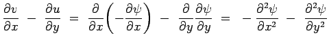 |
(4.61) |
Which leads to the condition that
 for
irrotationality. for
irrotationality.
Thus we see that the velocity potential automatically
complies with
the irrtotatioanlity condition, but to satisfy the continuity
equation it has to obey that
 . On the other
hand the stream function readily satisfies the continuity
condition, but to meet with the irrotationality condition it has
to obey
. . On the other
hand the stream function readily satisfies the continuity
condition, but to meet with the irrotationality condition it has
to obey
.
Thus we see that the streamlines too follow the Laplace Equation.
So it is possible to solve for a potential flow in terms of stream
function.
|
Property |
|
|
| Continuity Equation |
Automatically Satisfied |
satisfied if
 =0 =0 |
| Irrotationality Condition |
satisfied if
 =0 =0 |
Automatically
Satisfied |
Table 4.1: Properties of stream function and velocity potential
- 2
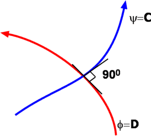
- Streamlines and equipotential lines are orthogonal to each
other. We have seen that the velocity components of the flow are
given in terms of velocity potential and stream function by the
equations,
Those familiar with Complex Variables theory will recognise that
these are the Cauchy-Riemann equations and that  and and
 are orthogonal and that both and obey
Laplace Equation. However, we will prove the orthogonality
condition by other means. are orthogonal and that both and obey
Laplace Equation. However, we will prove the orthogonality
condition by other means.
Figure 4.13: Orthogonality of Stream lines and Equi-potential lines
-
-
-
Since , it follows that
The gradient of the equipotential line is hence given by
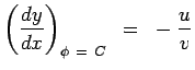 |
(4.64) |
On the other hand the gradient of a stream line is given by
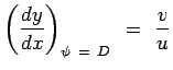 |
(4.65) |
Thus we find that
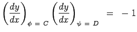 |
(4.66) |
showing that equipotential lines and streamlines are orthogonal to
each other. This enables one to calculate the stream function when
the velocity potential is given and vice versa.
Fig. 4.14 shows the flow through a bend where the
streamlines and the equipotential lines have been plotted. The two
form an orthogonal network.
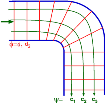
Figure 4.14: Stream lines and Equi-potential lines for flow through a bend
(c) Aerospace, Mechanical & Mechatronic Engg. 2005
University of Sydney
|