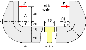
The cross-sectional depth of a thick curved beam is comparable to its radius of curvature and this gives rise to stress concentration. It is required to ascertain the variation of stress across the cross-section. Exact analysis is complex but the simple approximation which follows - based on plane cross-sections remaining plane under load - is adequate for most practical beams typified by the curved portion of the G-clamp illustrated.
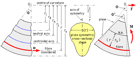
The generalised sector of a thick curved beam with centre of curvature at O and small angular extent Φ appears below. The radii of interest are identified in the LH sketch. Two radii are particularly significant - the mean (or centroidal) radius rc, and the mean reciprocal radius rd. They are defined by :
( 1 ) A * rc = ∫ riro dA * r ; A / rd = ∫ riro dA / r
Like ri and ro, both rc and rd are intrinsic to the known geometry ( b = f(r) ) of the cross-section.
Since the beam is curved, the radius defining the unstressed neutral axis, rn, is not immediately obvious as it would be in pure bending of a straight beam - it depends on the load and is unknown initially.
|
In the normal situation the resultants may be ascertained easily since they equilibrate other loads, which are usually known. Shear is neglected as in simple bending of a straight beam.
Application of M increases the curvature, so the angle subtended by the sector increases to Φ' under load in the RH sketch. Assuming that plane cross-sections remain plane during loading, the increase in length of the typical fibre at radius r is proportional to the distance from the unstrained neutral axis, ( r-rn). Since the original length of the fibre is proportional to the radius r, then :
fibre strain = extension/free length ∝ ( r - rn )/r = 1 - rn /r
Presuming elastic behaviour, the stress σ in the fibre at radius r is proportional to this strain, so
( 2 ) σ ∝ 1 - rn /r = σm ( 1 - rn /r ) where σm and rn are constants, as yet unknown.
This establishes the form of the stress variation across the cross-section; it is clear that the distribution is non-linear, giving rise to high stress magnitudes at small radii - that is, stress is concentrated where curvature is sharpest where r becomes small. Determination of the two constants follows from the necessity for the resultants of the stress distribution ( 2) to be the known F and M noted above. Thus, for equivalence of the distribution and the resultants, using ( 1) and ( 2) :-
F = ∫ A σ dA = σm ∫ A ( 1 - rn /r ) dA = σm A ( 1 - rn /rd )
M = ∫ A σ r dA = σm ∫ A ( 1 - rn /r ) r dA = σm A ( rc - rn )
Solving these for the two unknown constants :-
( 2 ) rn = rd ( M - F rc ) / ( M - F rd ) ; σm = ( M - F rd ) / A ( rc - rd )
It is noticed these two constants - and hence the stress distribution ( 2) - depend only upon the loading ( F & M) and the cross-sectional geometry ( A, rc & rd ).
Two particular locations of the neutral axis occur when
M = 0 whereupon rn = rc, and
F = 0 then rn = rd - the pure bending case most commonly encountered in the literature.
Summarising - application of the foregoing theory involves the following steps :
The conspicuous radii, rc & rd, for common symmetric cross-sections are found from ( 1) as follows.
Trapezoid - defined by dimensions ri , ro , bi and bo as sketched.
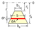
The variables r and dA must be expressed as functions of the same variable before the integrals in ( 1) can be evaluated. The radius r itself is the logical choice for independent variable, since, from the sketch dA = b.dr, where b is evidently linearly dependent on r, say
b = α + β r where the constants α and β are evaluated at ri and ro :
α = ( bi ro - bo ri ) / ( ro - ri ) ; β = ( bo - bi ) / ( ro - ri )
∴ dA = b dr = ( α + β r ) dr and therefore, from ( 1) :-
A = ∫ A dA = ∫riro ( α + β r ) dr = 1/2 ( ro - ri ) ( bi - bo )
A*rc = ∫ A dA*r = ∫riro ( α + β r ) r dr = 1/6 ( ro - ri ) [ bo( 2ro + ri ) + bi( 2ri + ro ) ]
A/rd = ∫ A dA/r = ∫riro ( α/r + β ) dr = bo - bi + [ ( biro - bori )/( ro - ri ) ] . ln ( ro /ri )
Rectangle - particularising the trapezoidal results with bo = bi = b ( constant ) :-

A = b ( ro - ri ) ; A*rc = 1/2 b ( ro2 - ri2 ) ; A/rd = b ln ( ro /ri )
Circle - integrating as above :- 2 rc = ro + ri ; 2 √rd = √ro + √ri
Built-up sections
 may be analysed by dividing them into a number of simple shapes for each of which the integrals in ( 1) are calculable, then applying ( 1) in discrete form :-
( 1a ) A = Σj=1 ( δA )j ; A*rc = Σj=1 ( δA*r )j ; A/rd = Σj=1 ( δA/r )j
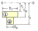
Consider the T-section shown, consisting of two rectangular elements :-
| element | width | inner radius | outer radius | δA | δA*rc | δA/rd |
| 1 | bi | ri | rm | bi ( rm - ri ) | 1/2 bi ( rm2 - ri2 ) | bi ln ( rm/ri ) |
| 2 | bo | rm | ro | bo ( ro - rm ) | 1/2 bo ( ro2 - rm2 ) | bo ln ( ro/rm ) |
| total | Σj=1 ( δA )j | Σj=1 ( δA*r )j | Σj=1 ( δA/r )j |
The most heavily stressed cross-section is assumed to be just to the left of A-A as shown, since
Section properties :
From the above T-section results with ri = 20, rm = 30, ro = 50, bo = 15, bo = 5 mm :
A = 15 ( 30 -20) +5 ( 50 -30) = 250 mm2 watch units!
A*rc = [ 15 ( 302 -202 ) +5 ( 502 -302 ) ]/2 = 7750 mm3 whence rc = 31 mm
A/rd = 15 ln 30/20 + 5 ln 50/30 = 8.636 mm whence rd = 28.95 mm
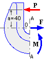
The stress resultants, F and M, are shown on the free body in the conventional positive senses used in developing the theory above. For equilibrium of the free body, F = P and M = -Pa. Inserting these into ( 3) gives :-
rn = rd ( a + rc )/( a + rd ) = 28.95 ( 40 + 31 )/( 40 + 28.95 ) = 29.81 mm
σm = -P ( a + rd )/A ( rc - rd ) = -750 ( 40+28.95)/250( 31-28.95) = -101 MPa
The stress distribution is thus σ = -101 ( 1 - 29.81/r ) MPa where r is in mm.
The stress distribution is plotted
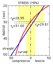 and yields extreme values of 49 MPa tensile at the inside (20 mm radius), and 41 MPa compressive at the outside. As the stress nowhere exceeds 50 MPa, the claimed capacity seems vindicated.
But, for the straight portion :-
I = 15 ( 103/12 +10*62 ) + 5 ( 203/12 +20*92 ) = 18083 mm4, so
σ = σd + σb = P/A + My/I
= 750/250 - 750(40+31).( r -31)/18083 = 3 - 2.945 ( r -31) MPa
This stress distribution also is plotted and indicates a tensile stress of 35 MPa at the inside, and 53 MPa compressive at the outside. The clamp is therefore some 6 % under-designed and unsafe. But it is physically impossible for two distinct stress distributions to occur at an infinitessimal distance apart across the interface A-A. The actual distribution at A-A will therefore lie somewhere between those found - however this does not invalidate the conclusions regarding clamp inadequacy . . . . why ?