Kinetics

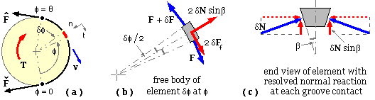
The equations of motion for the elemental free body travelling at constant belt speed v, from (b) are
tangentially :     ( F + δF ) cos ^δφ/₂   - F cos ^δφ/₂   - 2 δF_f   =   0     since there is no angular acceleration
normally :           ( F + δF ) sin ^δφ/₂  + F sin ^δφ/₂   - 2 δN sin β   =   δm.a_n   =   ( ρ . rδφ ).( v² /r )   =   ρ v² . δφ
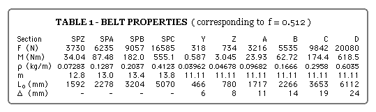
                                      where   ρ is the belt's   linear density (kg/m), a belt property - see Table 1.

In the limit these two equations yield :       dF_f / dN   =   dF. sin β / ( F - ρ v² ). dφ
Furthermore, if gross slip is to be avoided then   dF_f / dN   ≤   μ     the coefficient of belt/groove friction.
Eliminating   dF_f / dN here, separating variables, and integrating over the contact arc   0 ≤ φ ≤ θ :-

( i)     ( F_max - ρv² ) / ( F_min - ρv² )   ≤   e ^{( μ cosec β ) θ}

This relation specifies the maximum ratio of belt tensions which a given belt/pulley interface can support without gross slip. The   ρv² term, often conveniently if erroneously referred to as the   centrifugal tension, detracts from the interface's useful tension ratio capabilities. It is convenient to define   f ≡ μ∗cosec β as the   effective coefficient of friction which reflects the amplification of the actual coefficient   μ   by wedging action in the groove of angle   β.

A drive comprises two pulleys, potentially with different values of   μ, β, and θ   - although the slack and tight strand tensions are common to both pulleys. The maximum tension ratio which the drive can support without slip on   either of the two pulleys is therefore :

( 3)     ( F_max - ρv² ) / ( F_min - ρv² )   ≤   e ^{( f θ)_min}
                                    where   f ≡ μ∗cosecβ     and   ( f θ)_min   =   min (   (fθ)₁ , (fθ)₂ )

If   f is the same for both pulleys, as is usual when both pulleys are grooved, then the smaller pulley will be limiting since   θ₁ < θ₂ , but this does not necessarily apply to   V-flat drives   (see below).

A representative coefficient of friction is 1/6, and this together with a wedge angle   2β = 38^o and a wrap angle of   180^o in a 1:1 drive, corresponds to a static tension ratio   F_max /F_min =   e^0.512π =   5.0

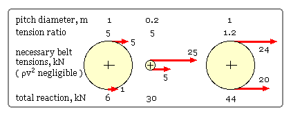
The effects of tension ratio and pulley diameter on loads generally may be appreciated by the three pulleys in 1:1 drives illustrated here, all of whose torque capacities are   2 kNm. The second pulley is one fifth the diameter of the first, so the forces have to be five times those of the first for the same torque - clearly this has severe repercussions not just on belt loading but also on shaft bending, bearing reaction etc. The third pulley is the same as the first however the tension ratio is much smaller due to a reduced RHS of ( 3) - again larger forces occur right throughout the drive train.

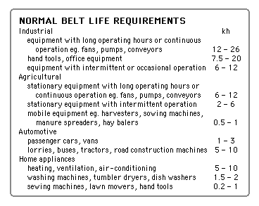
Large pulleys and tension ratios are clearly beneficial, however tension ratios are limited by the friction coefficients and wrap angles which are encountered in practice. Attempts are sometimes made to increase drive capacity by increasing the initial tension, but if belts are overtightened then their fatigue lives will suffer, though by how much we cannot say, since the foregoing model ignores initial tension except insofar as "normal" tightening practice is assumed. Whilst large pulleys reduce loads and hence the cost of mounting shafts and bearings, the initial cost of the pulleys themselves increases with size. So the design of a power transmission train in practice needs to be carefully balanced from an economic point of view. The manufacturers of electric motors recommend minimum pulley diameters for acceptable motor bearing lives   ( see tutorial problems ).

Every cross-section of the belt is subjected alternately to the strand tensions   F_max and   F_min and therefore undergoes fatigue. These tensions at least must be detemined before fatigue can be addressed. If the power transmitted by the drive   P is shared equally between   z belts in parallel then since the torque per belt always equals   ( F_max - F_min) ∗ radius :-

( 4a)       P   =   z ( F_max - F_min) v       ie.       F_max - F_min   =   P / z v

This relation alone is insufficient for determining   F_max, F_min individually for a given power- per- belt (P/z) and velocity (v). If however we focus on the maximum power transmissible without gross slip, then   equation ( 3) applies. Eliminating   F_min between ( 3) and ( 4a), the tight side tension   F_max per belt for a given slip- limited power P is :-

( 4b)       F_max   =   P / z k_θ v   + ρ v²     where the drive property     k_θ ≡ 1 - e ^{- ( f θ)_min}     by definition.

It must be emphasised that although ( 4a) is always relevant, equation ( 4b) applies only when slip is imminent, and relates to the maximum power capacity of the drive, dictated by slip on the more susceptible pulley. At part load, when slip is not limiting, it is common practice to deduce approximate tensions from the full- load ratio given by ( 3), together with the tension difference corresponding to the actual part- load torque from ( 4a)   ( see the tutorial problems ).

Fatigue

The sketch here illustrates the qualitative variation of equivalent force on a belt element as it passes the points 1-2-3-4 of the above geometric sketch. 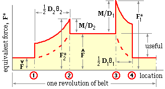An element in the slack side straight encounters the large pulley at 1, the tension in the element thereafter increases due to friction over the arc of contact   θ₂ , the equivalent damaging force in the element is increased also by   M/D₂ . When the element leaves the pulley at 2 the bending term no longer applies and the element's load is merely the tight side tension   F_max   { nomenclature explanation}. The reverse process occurs as the element passes around the smaller pulley, the element tension returning to   F_min after 4.
Each element evidently undergoes a double- peaked fatigue cycle during one revolution of the belt. Since   D₁ ≤ D₂ it follows that the   F₁* peak cannot be less than the   F₂* 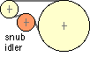peak. A snub idler, that is an idler located on the outside of the belt to increase the arc of contact on the small driveR, should normally be avoided since it introduces reversed bending and hence increases the stress range markedly.

It is required to determine the belt life under this double- peaked fatigue cycle.
 

For many cyclically loaded components, including belts, there exists an approximate log-log linear relationship between :

-	the load on the component, characterised by the equivalent damaging force   F* in the case of a belt, and
-	the life of the component   N* at failure (expressed in cycles of load application), viz :-

        life ∗ load^index   =   constant       or, for a belt       N*   =   ( F / F* ) ^m
              in which both the index   m and the reference load   F are constant properties of the belt ( Table 1 ).

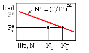A belt subjected only to the force varying between zero and   F*_i will fail after   N*_i cycles as sketched. At a certain point in time prior to failure it will have undergone   N_i cycles, so the   cumulative fatigue damage at that instant may be taken as   N_i /N*_i. Thus when the load is first applied   N_i ≈ 0 and no appreciable damage has occurred; when   N_i ≈ N*_i   damage is almost 100% and so failure is imminent.

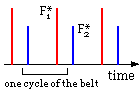
In a drive situation a belt is subjected essentially to a cycle comprising two peaks of magnitude   F*₁ and   F*₂. If the life of the belt under these combined loads is   N_c then   Miner's rule states that failure occurs when the cumulative damage via both mechanisms reaches 100% - that is :
        N₁ /N*₁ + N₂ /N*₂   =   1       where by the nature of loading :   N₁ = N₂ = N_c
The effects of further pulleys could be incorporated if appropriate at this point.

The elapsed time for one such belt cycle is   L/v, so the drive life   T in units of time   ( not to be confused with torque ) is   T = N_c L/v. Substituting for the lives   N*_i via the load-life equation and for the loads   F*_i from ( ii) leads to the desired result :-

( 5a)         Σ _{i = 1,2} (   P/z k_θv + M/D_i + ρ v² ) ^m   =   F^m ( L/vT )

This is the final design equation for the drive - like all design equations it relates the four major aspects :

	load	power per belt (P/z), velocity (v)
	dimensions	pulley diameters (D1 , D2 ), belt length (L) and friction/arc factor (kθ)
	material	ie. belt section and corresponding properties (F, M, ρ, m) from Table 1
	degree of safety	or more appropriately in a fatigue situation, the drive life (T)

Properties found by curve fitting to belt capacities cited in the Code, are given in Table 1. The design equation appears to be a relatively sophisticated model, but it is important to realise that most of the sophisitication lies in the arithmetic since the model is based upon some rather gross assumptions, including :-

• neglect of significant 3-D stressing, apart from bending and direct tension, as indicated below by distortion of cross-sections due to pulley contact and the tensile members
• the complete disregard of initial tension and tension variation between belts
• non-metallic materials may not follow the stress/strength theories applicable to metals, and will probably not behave elastically
• the inexactness inherent in any fatigue analysis, and in particular, the questionable accuracy of Miner's rule
• probable operation of the drive at less than its gross- slip- limited capacity
• neglect of the tendency for the belt to ride out of the groove as its tension reduces, so increasing the pulley's effective pitch diameter
• variations in the coefficient of friction
• neglect of transients such as high starting torques
• the composite nature of the belt, with components having different load-life relations, etc.

( 5b)       P_π   =   k_π v [   F ( L/2vT )^1/m   - M/D   - ρ v² ]   ;       where   k_π ≡ 1 - e^-fπ

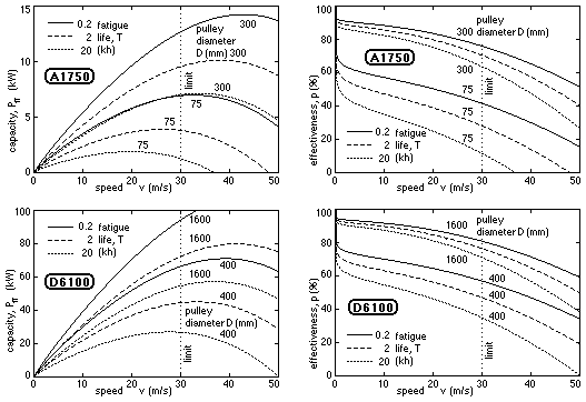The variation of capacity with velocity is plotted here for two typical V-belts - A1750 and D6100. Effectiveness is explained in the next section.
The capacity is evidently a fatigue- limited value which depends upon the belt size and which decreases as the fatigue life increases (ie. the first term on the RHS of ( 5b)) - this value being reduced by bending and by centrifugal effects (the second and last terms on the RHS). Large pulleys clearly improve belt capacity, though the reciprocal nature of the bending term means that increasing the diameter of a pulley which is already large may have little effect on belt capacity. Centrifugal effects cause the capacity to peak and eventually to decrease with increasing speed.

Effectiveness

( 5c)       ( p + b₁ + c )^m + ( p + b₂ + c )^m   =   2   ;     where   p   =   ( P / Fk_θvz ) ( 2vT/L )^1/m

The three terms in each bracket of this equation represent the fractional consumption of finite fatigue life by useful power transmission, and by deleterious bending and centrifugal effects respectively. The first term,   p, is interpreted as the   effectiveness of life usage. If bending and centrifugal effects are negligible then the majority of the life is devoted to power transmission and the effectiveness approaches 100%. If, on the other hand, bending or centrifugal effects predominate, then the belt is not being used effectively and a low value of p results. Effectiveness should not be confused with efficiency.

The effectiveness of the two belts graphed above illustrates a monotonic drop- off with increasing speed, and effectiveness is reduced markedly by increased bending over small pulleys. Lacking costs, effectiveness may be used to assist in the selection of the optimum drive for a given duty. Drives cited in manufacturers' brochures correspond to values between about 30 and 70%.

Drive selection

• the power capacity of the drive and the small pulley's shaft speed (rev/s)
• acceptable limits of the speed ratio   R - though it is common for only a single nominal speed ratio to be specified, around which the designer must set bounds commensurate with the duty
• limits of pulley centre distance - once again the designer may have to define a tolerable band around a sole nominal value or, lacking even this, around 2D₁ √( R+1)
• limits of acceptable belt fatigue life: it is rare for these to be stated explicitly, and the designer may have to adopt limits in line with the duty (see the table here) and economic belt replacement frequency, or with the usual commercial expectation of 26 kh.

Drive selection involves choice of size (B, SPA etc) number and pitch length of the belt(s), and diameters of the two pulleys. As the design equations cannot be solved in closed form, and since many parameters are discrete, a trial- and- error selection process must be adopted. The steps illustrated below form a useful framework for this, and should be read from top to bottom.

The process starts with the choice of a suitable belt size - aided 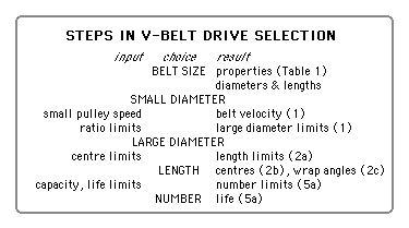by a carpet diagram - with belt properties from Table 1 and with corresponding lists of readily available belt lengths and pulley diameters. The smaller pulley diameter is next selected, and is usually taken as small as possible to reduce potential pulley costs - consistent with acceptable belt life and effectivness. Belt speed and bounds on large pulley diameter follow from the desired speed ratio limits and equations ( 1) ie.   R_min D₁ ≤   D₂ ≤   R_max D₁ .

If feasible, a large pulley   D₂ is next chosen from the diameters available within this range, and belt pitch length limits   L_min , L_max corresponding to the stated centre distance limits   C_min , C_max worked out from ( 2a). If feasible, a belt length   L_min ≤   L ≤   L_max is next chosen from the lengths available, and the geometry finalised via ( 2b), ( 2c).
The sole design parameter which now remains to be chosen is the number of belts,   z. Rather than follow the schema by working out limits to the number of belts consistent with stated life constraints, it is probably easier just to choose various belt numbers on a trial- and- error basis and evaluate belt life from ( 5a) until a suitable life eventuates.

This process is repeated with different initial choices of belt size and small pulley diameter, to provide a bank of solution candidates with acceptable lives. Selection of the 'best' solution is based thereafter upon economic considerations. The drive-selection program V-belts operates in this way, with nested loops corresponding to belt size, small pulley diameter etc, as in the schema above. Users should check that belt lengths and pulley diameters cited by it are available locally. V-belts is capable of handling V-flat drives (see below) as may be seen from the appended dialogue, and alerts if the aforementioned speed limits are exceeded or if dynamic balancing of the pulleys is necessary.

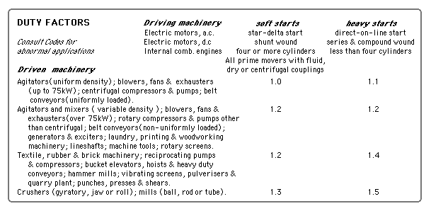
The design power input to the selection process must incorporate a duty factor to allow for shock, high starting torques and other expected non-uniformities :-

( iii)       design power   =   actual nominal power ∗ duty factor (from the table below eg.) Note that a duty factor of 1.5 implies a life reduction of approximately   1.5¹² = 130.

Codes and belt suppliers' literature do not employ the design equation ( 5a) directly, but present instead a selection procedure based on charts and factors which are derived from approximations to the design equation. Since we cannot always have software like V-belts to hand, it is advisable to be conversant with these approximate solutions.