DANotes: Springs: Fatigue analysis

strength v. diameter for ferrous spring materials

Wire materials

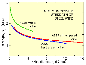
The majority of springs are cold wound from cold drawn carbon steel. The marked increase of tensile strength S_ut with decreasing wire diameter d is graphed for three common steel wires - the corresponding expressions in Table 2 below which relate strength to diameter are regressions for data in the Spring Design Manual (op cit) which may be consulted for data on other materials.
The strength ratios in Table 2 were prepared from graphs presented by Godfrey showing allowable shear stress limits for different wire diameters and materials. Strengths are :

- S_us	ultimate strength in shear
- S_ys	yield strength in shear - permanent set results if this is exceeded
- S_es	fatigue strength in reversed shear corresponding to 10 Mc (10⁷ cycles).

The ratios are lower bounds to Goodman correlations of experimental fatigue data from various workers for a large number of springs with typical surface finishes. Godfrey includes also plots for lives other than 10 Mc, from which the corresponding fatigue strengths may be deduced.

TABLE 2 - PROPERTIES OF FERROUS SPRING WIRE
material	hard drawn wire	music wire	oil tempered wire
designation	ASTM A227/SAE J113	ASTM A228/SAE J178	ASTM A229/SAE J315
nominal carbon, %	0.5 - 0.8	0.7 - 1.0	0.6 - 0.8
common sizes (d) mm	0.5 - 12.5	0.2 - 5	0.8 - 16
general attributes	cheapest; not for fatigue due to surface defects	best quality; especially for smaller springs	general purpose but fatigue life limited
tensile ult. (S_ut) MPa	2470 +d( 2910 +40d)	3370 +d( 6560 -230d)	2630 +d( 2180 +56d)
tensile ult. (S_ut) MPa	1 +d( 2 +0.1d)	1 +3.5d	1 +d( 1.6 +0.08d)
S_us / S_ut	0.52	0.50	0.63
S_es / S_ut	0.13	0.15	0.13
S_ys / S_ut	0.43	0.43	0.48

Fatigue applications such as engine valves demand a high surface finish of the wire, so the choice of material is based largely on this characteristic which is a result of the method of wire manufacture. Expensive care is taken to maintain the surface of valve spring quality (VSQ) wire free from defects.

Presetting and shot peening

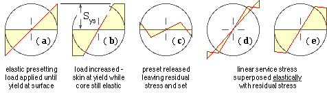
Presetting (or "scragging") and shot peening are two manufacturing operations which are carried out after coiling and heat treatment, but before putting a spring into service. They each confer a favourable residual stress distribution in the wire which increases the allowable operating loads.

The stresses in a torsion bar made from an elastic-perfectly plastic material during and after presetting are sketched here. A relatively large presetting load (torque) is applied to cause a band of material under the surface to become plastic while the core of the wire remains elastic ( b).
presetting a torsion bar
When the presetting load is removed the bar recovers elastically but does not return to its original position since part of the wire cross-section has yielded - the bar remains permanently deformed. The corresponding residual stresses ( c ) are negative at the surface - negative in the sense of the stress induced by the applied load. When the bar is subsequently put into service these residual stresses are elastically subtractive from the stresses attributable to the load ( e), so that surface stresses are less than those which would have occurred in the absence of preset. A more detailed explanation of presetting is given in the Appendix.
Presetting a spring, as opposed to a torsion bar, involves making the spring sufficiently long so that portion of the cross-section yields when the spring is compressed solid during preset. When the presetting load is removed the spring recovers elastically to a shorter free length. The residual stresses are similar to those in a torsion bar, but more complex due to direct shear and curvature-induced stress concentration. Presetting usually reduces the stiffness by 5-10%.

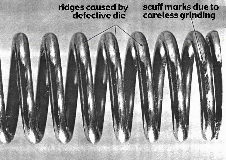
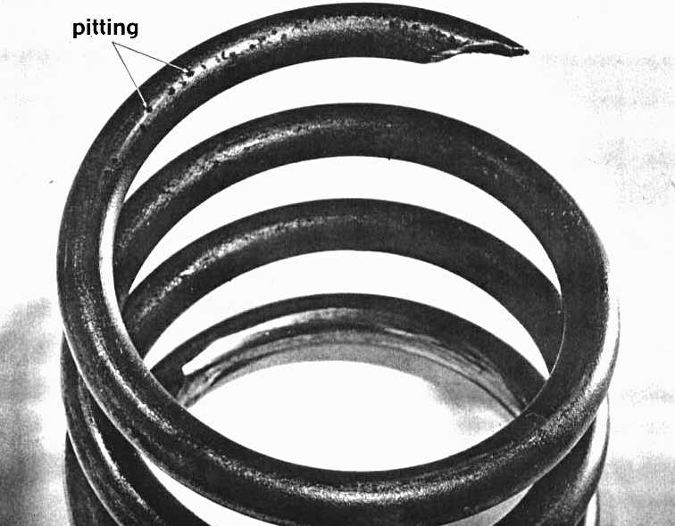
Shot peening involves bombarding the wire with high velocity pellets to impart a surface compression. Residual stresses are more surface- localised than those induced by presetting. Peening is particularly beneficial for fatigue in the presence of surface flaws (die marks, pits and seams), but is appropriate only for wire diameters exceeding 1.5 mm or thereabouts.
Springs destined for arduous duty are invariably preset and/or peened, however in the interests of simplicity we shall not make use of the significantly higher design stresses which these operations allow. The material strengths tabulated above refer to springs without preset or peening.

Fatigue loading

If a compression spring is designed with the yield limit above the solidity limit and manufactured correctly then the only way it can fail is through fatigue. The leftmost photograph of a typical fatigue failure surface reveals a crack source near the inner more highly stressed surface of the wire. If stress raisers occur due to poor manufacture or to corrosion as illustrated in the other photographs, then fracture is likely to emanate from the stress raisers thereby reducing fatigue life.

In the absence of such stress raisers, correlation of the repeated loading on a spring with its material's properties in order to ascertain safety is usually carried out via a Goodman analysis. Given the spring material and wire diameter, the shear ultimate S_us and fatigue strength in reversed shear S_es may be found from the literature, or as explained above. 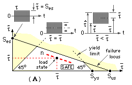figure A The conservatively straight Goodman failure locus is thus defined in τ_a - τ_m space, as shown on the diagram ( A) { nomenclature explanation}.

Spring loading is almost invariably unidirectional, so τ_a ≤ τ_m and loading states occur only to the right of the 45^o stress equality line. One such load state is illustrated, lying on a line which corresponds to a safety factor of n, ie. the line joins the points ( S_us/n, 0), (0, S_es/n) and so lies parallel to the failure locus. From similar triangles the Goodman fatigue equation is :

( 4a) τ_m/S_us + τ_a/S_es = 1/n in which the stress components are given by
τ_m = K_s 8 F_mC / πd² where F_m = ( F_hi + F_lo) /2 and
τ_a = K_h 8 F_aC / πd² where F_a = ( F_hi - F_lo) /2

The full stress concentration factor K_h is applied to the alternating component τ_a in ( 4a). Stress redistribution is presumed to follow localised yielding, with the result that stress concentration is usually ignored in figuring the steady component of fatigue loading. The mean stress τ_m is therefore based on the factor K_s, which accounts only for direct stresses in the torsion equation.

The safe operating window of the Goodman diagram is completed by the yield limit. If n_y is the factor of safety against the yield being exceeded, then :

( 4b) τ_m + τ_a = S_ys/n_y since ( τ_m + τ_a) represents the maximum stress.

A fatigue analysis of the preceding example using ( 4a) is carried out in this example.

The traditional method of presenting allowable fatigue stresses is to plot the maximum shear stress τ_hi against the minimum τ_lo, rather than the amplitude versus the mean as above. Although strictly not correct, the full stress concentration factor K_h is applied conservatively to both components which are inserted into the Goodman expression ( 4a) to give the failure locus:

( 4c) τ_hi = { 2 S_usS_es/ ( S_us + S_es) } + { ( S_us - S_es) / ( S_us + S_es) } τ_lo where
τ_hi = K_h 8 C F_hi / πd² and τ_lo = K_h 8 C F_lo / πd²
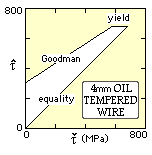
Thus for the wire of the foregoing example with stresses in MPa :

( 4a) Goodman failure locus τ_m/888 + τ_a/183 = 1
( 4b) yield failure criterion τ_hi = 677
( 4c) modified Goodman locus τ_hi = 303 + 0.658 τ_lo

Though ( i) and (iii) appear identical, since τ_hi = τ_m + τ_a and τ_lo = τ_m - τ_a, the four stress components are defined with different stress factors in ( 4a) and ( 4c). The safe operating window from the last two relations is shown here. States below the equality line are impossible as this would mean reversal of the minimum / maximum roles. The material strengths of Table 2 were deduced via ( 4c) from plots such as this in Godfrey.

The fatigue strength in repeated (one-way) shear S'_es forms the basis of a Goodman approach, diagram ( B) which is less conservative than that based on reversed shear, diagram ( A). 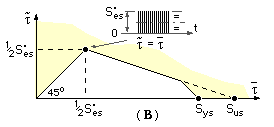figure B If the test stress varies between zero and S'_es, then τ_a = τ_m = S'_es/2, and the failure line joins the points ( S_us, 0), ( S'_es/2, S'_es/2 ). The resulting design equation is :

( 4d) τ_m/S_us + τ_a( 2/S'_es - 1/S_us) = 1/n

Since it is rare that the fatigue strength in repeated loading is available, we will henceforth employ ( 4a) and ( 4b) with the fatigue strength corresponding to whatever life is of interest.