WELDED JOINTS

In arc welding an electric arc at the extremity of a travelling consumable electrode maintains a pool of molten metal in which the components and electrode material coalesce, forming a homogeneous whole (ideally) when the pool later resolidifies. But no joint can be perfect, and it is the designer's job to allow for practicalities and to ensure that the joint is adequate and economical.
The materials of components and electrode must be compatible from the point of view of strength, ductility and metallurgy - this last being most important in view of thermal effects arising from the usual uncontrolled localised cooling. The various Codes lay down electrodes which should be used for given steels - AS 1554 eg. cites electrode classification E41xx as first preference and E48xx as second, when welding steel grades 250 through 350 - the number in the classification being one tenth of the deposited weld metal's ultimate tensile strength (MPa).

The form of a welded joint is dictated largely by the layout of the joined components; the two most common forms are the butt and fillet joints illustrated.

A butt weld aims usually for full penetration with no voids in the completed joint, so edge preparation to allow electrode insertion is required for all but the thinnest weldable components. Inhomogeneities may be minimised by double welding (ie. welding from both sides as sketched), by ultrasonic examination with subsequent repair if necessary, or by other means. In non-critical applications, correctly fashioned butt joints carried out by competent welders are often taken to be just as strong as the joined components - that is, provided the electrode is correctly chosen and the welding technique is satisfactory then joint safety does not have to be separately addressed. But the occurrence of imperfections in potentially hazardous joints must be recognised and allowed for in design, as will be seen later in the context of   Pressure Vessels.

The majority of the deposited material in a fillet weld lies outside the silhouette of the joined members; penetration is not complete and a crack is inherent. The weakening effect of cracks are examined under   Fracture Mechanics, but it is immediately obvious that the geometric singularity at the end of a crack could not be more extreme and so severe stress concentration in the fillet is inevitable. Fillet welds with their intrinsic cracks are never specified if fatigue loading is substantial.

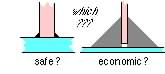
While the dimensions of a butt joint are governed in the main by the thickness of the joined components, the size of a fillet weld is not limited by component thickness except for reasons of heat transfer and resulting weld quality. But do either of the two fillets illustrated here   look practicable ?
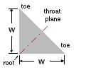
The weld cross-section is idealised as a 45^o fillet whose size is characterised by the dimension   w - only welds of constant size are considered here. The locus of fillet centroids (or roots, approximately) traces out the weld run of length  L. The run may be continuous or discontinuous. Since the run's shape is dictated largely by the joined components, the only means of varying the load capacity for a given electrode material is to vary the size   w.

Successful welds depend as much on practical issues as on on theory. It is not the present intention to dwell on practicalities - the reader is referred instead to the Bibliography for advice on practical necessities.   AWRA Technical Note #8 illustrates many important considerations and is required background to the serious design of welded joints. However there is one simple issue which should be appreciated at the outset - the cost of a weld is approximately proportional to the amount of electrode used, other things being equal. The welds on the right here are obviously more expensive than those on the left - but by how much in relative terms ?

So, the size of a fillet weld must be sufficiently large for safety, without being so large that unnecessary expense is incurred. Clearly a rational design procedure for such joints is needed - one based upon the steps already identified : resolution of indeterminacies, load building blocks, stress resolution and implementation of an appropriate failure theory. The derivation and application of such a procedure is the main thrust of this chapter.

Fillet welded joints

In general the resultant load on the joint is a force   F = [ F_x F_y F_z ]' through the centroid of the linear run, together with a moment   M = [ M_x M_y M_z ]'   whose components are given by the RH Rule, ( b). For the cantilever above, this resultant would be found by moving the sole force to act through the centroid, and introducing the moment corresponding to the force multiplied by the distance transverse to the force's line of action between the point of load application and the centroid.

This load is equilibrated by a force distributed along the length   L of the run as indicated in ( c). By virtue of the stresses in the weld, each element of run   δL contributes an elemental force   q.δL towards equilibrium. q is a force intensity ; it is a vector force -per -unit -length and except in simple cases varies in magnitude and direction around the run.
Conceptually, force intensity is not too different from stress, which is a force -per -unit -area, that is   δF = q δL = σ δA. Force intensity is also similar to the bending moment in a beam: both are stress resultants - of stresses in the weld throat and in the beam's cross-section respectively - and both vary in general along a linear path - the weld run and the beam axis.

For the majority of beams the bending moment is easily found in terms of the loads using statics. In the case of a fillet weld however, correlating the intensity   q with the load   F, M is less straightforward since the arrangement is statically indeterminate.
Two techniques for this correlation (having the same theoretical foundation) are presented below. The first traditional approach is based on recasting the building block stress equations for bending etc. in terms of force intensity rather than of stress. This approach though simple has limitations which in some situations requires the more general second technique, the unified approach.

Geometric properties of lines

It is useful to review the concepts of centroids and second moments of linear though not necessarily straight runs, ie. of lines rather than of areas. Two dimensions only are detailed, however the underlying concepts may be extended to three dimensions.

The geometry of the planar line ABC shown here is known. The line's centroid is found by first erecting any convenient (X,Y) Cartesian system in the plane, then applying first moments (Varignon's Theorem) to all line elements   δL. The centroid's abscissa   X_G may be defined in alternative ways :

( i)	Σ XG δL	=	Σ X δL		more usually seen as   XG   =   ( Σ X δL )/L     or, collecting terms
	Σ ( X - XG ) δL	=	0		or, shifting the Cartesian origin to the centroid and setting   x = X-XG
	Σ x δL	=	0		which in the limit becomes   ∫L x dL = 0
		that is, the centroid is that point about which the first moment of length vanishes.

Extending this argument to three dimensions leads to the conclusion that the centroid is that unique point for which all components of first moments vanish :   Σ x.δL = 0,   Σ y.δL = 0,   Σ z.δL = 0   or, in brief   Σ r δL --> ∫_L r dL = 0   where   r = [ x y z ]'. The above run ABC lies in the   z = 0 plane.

The sum-of-increments approach is extended to higher moments, thus the second moment of a line about a defined axis is :
      I_axis   =   Σ_{over all elements} { ( length δL of each element ) ^_* ( the element's distance from axis )² }

                -->   ∫_L ( distance of dL from axis )² dL

Integral forms are suitable for continuous line segments for which the geometry   f(x,y,z) = 0 is known; discrete forms are suitable in conjunction with the Parallel Axes Theorem for a line made up of a number of segments whose individual centroids and second moments are known from tables for example, or from the useful results of Tutorial Problem 6.
Properties of some common run geometries are tabulated here; it should be noted that :   O [ second moment of length ] = length ^_* distance² = length³. It is apparent that the process of finding centroids and second moments of lines is identical to that for areas - essentially it's a matter merely of interchanging   δL and   δA in the appropriate formulae.